Interpolated Sampling Mode
This topic describes interpolated retrieval mode. It also presents concepts that are common to interpolated, lab, calculated, and trend retrieval modes. Interpolation is a separate sampling mode and is also used in the various calculation modes.
Data compression necessitates interpolation. A minimal number of real data points is stored in the archive. On retrieval, interpolation is performed to produce an evenly spaced list of the most likely real world values. Even if you are not using compression, you can use interpolation if you want samples spaced on intervals other than the "true" collection rate.
The following data is used in the examples below. You can import this data into Historian if you want to try the examples yourself:
*Example for Interpolated Data Documentation
*
[Tags]
Tagname,DataType,HiEngineeringUnits,
LoEngineeringUnits TAG1,SingleFloat,60,0
BADDQTAG,SingleFloat,60,0
[Data]
Tagname,TimeStamp,Value,DataQuality
TAG1,29-Mar-2002 13:59:00.000,22.7,Good
TAG1,29-Mar-2002 14:08:00.000,12.5,Good
TAG1,29-Mar-2002 14:14:00.000,7.0,Good
TAG1,29-Mar-2002 14:22:00.000,4.8,Good
BADDQTAG,29-Mar-200213:59:00.000,22.7,Good
BADDQTAG,29-Mar-2002 14:08:00.000,12.5,Bad
BADDQTAG,29-Mar-2002 14:14:00.000,7.0,Bad
BADDQTAG,29-Mar-2002 14:22:00.000,4.8,Good
Timestamp
All sampling and calculation modes (except raw sampling) use the same method for creating intervals from the start and end time. Raw retrieval has no intervals, only a start and end time. Each mode differs in how it arrives at the value to assign to that interval
The simplest case is when the interval is evenly divisible by the number of samples or by the interval in milliseconds. For example, the start and end times are one hour apart and you want data at ten-minute intervals, or 6 samples. The first time stamp occurs at the start time + one interval and represents the samples from a point greater than the start time to less than or equal to the interval time stamp.
Example: Determining interval timestamps for evenly divisible duration
- Import this data into the Historian. There is only a tag, with no data.
[Tags] Tagname,DataType,HiEngineeringUnits,LoEngineeringUnits c1,SingleFloat,100,0 - Retrieve data for that tag over a 1-hour duration with a 10-minute interval. Use the following query:
select timestamp from ihrawdata where timestamp >= 14:00 and timestamp <= 15:00 and tagname = c1 and
numberofsamples = 6
or this query
select timestamp from ihrawdata where timestamp >= 14:00 and timestamp <= 15:00 and tagname = c1 and
Intervalmilliseconds = 10M
Both SQL queries result in the same intervals and interval timestamps
3/29/2002 14:10:00
3/29/2002 14:20:003/29/2002 14:30:00
3/29/2002 14:40:00
3/29/2002 14:50:00
3/29/2002 15:00:00
When the 1-hour duration is not evenly divisible, interval timestamps will include milliseconds even if the data samples do not use a resolution of milliseconds.
Example: Determining interval timestamps for a non-divisible duration
Divide the one hour duration from previous example into 7 intervals:
select timestamp from ihrawdata where timestamp >= 14:00 and timestamp <= 15:00 and tagname = c1 and
numberofsamples = 7
3/29/2002 14:08:34.285
3/29/2002 14:17:08.571
3/29/2002 14:25:42.857
3/29/2002 14:34:17.142
3/29/2002 14:42:51.428
3/29/2002 14:51:25.714
3/29/2002 14:59:59.999Value
- Attribute samples to intervals
- Any raw sample is attributed to exactly one interval based on the raw sample and interval time stamp. The rule is that the sample has to have a time stamp greater than the interval start time, but less than or equal to the end time. This is because the end timestamp of the interval is the start timestamp on the next interval.
- Interpolate a value at each interval end time
- For each interval end time, find the raw point before and after the end time. The interval time stamp is the interval end time; we can then interpolate the value at that time.
Example: Determining interval interpolated value
This example shows how linear interpolation determines the most likely real world value at the interval timestamp.
Using the same data set as above, there are raw points at:
14:08:00.000,12.5,Good
14:14:00.000,7.0,Good
and you are trying to get an interpolated value at 14:10. The calculation used for linear interpolation would be:
interpolated value = previous raw sample + ((deltaY/deltaX) * offset)Substituting the numbers for this example:
deltaY = 7.0 12.5 = -5.5
deltaX = 14-8 = 6
offset = 2 seconds (from 14:08 to 14:10)
Interpolated value = 12.5 + ((-5.5/6)*2) = 10.67
- About Interpolated Data Type
- When interpolating data, the data type of the value will be the same data type as that of the tag's raw data. Only floating point and double floating point values can be interpolated. Integers, strings, and blobs cannot be interpolated. When attempting to interpolate string and integer data, interpolation will simply repeat the collected value for each interval until the next collected value.
Example: Retrieving interpolated values of an interval with GOOD data
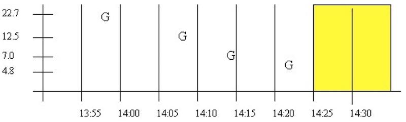
The raw samples for TAG1 can be plotted as follows. The ?G indicates a good data quality raw sample.
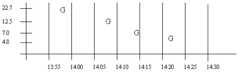
Use this SQL query to retrieve the data:
select timestamp, value, quality from ihrawdata where samplingmode=interpolated and timestamp >=
'29-Mar-2002 13:50' and timestamp <= '29-Mar-2002 14:30' and tagname = tag1 and numberofsamples = 8| Timestamp | Value | Quality |
|---|---|---|
| 29-Mar-2002 13:55:00.000 | 0.00 | 0.00 |
| 29-Mar-2002 14:00:00.000 | 21.57 | 100.00 |
| 29-Mar-2002 14:05:00.000 | 15.90 | 100.00 |
| 29-Mar-2002 14:10:00.000 | 10.67 | 100.00 |
| 29-Mar-2002 14:15:00.000 | 6.73 | 100.00 |
| 29-Mar-2002 14:20:00.000 | 5.35 | 100.00 |
| 29-Mar-2002 14:25:00.000 | 4.80 | 100.00 |
| 29-Mar-2002 14:30:00.000 | 4.80 | 100.00 |
There may be many raw points in an interval, but interpolation uses only the last one in the interval and the first one in the next interval. The sections below describe the interpolation behavior in the 3 possible cases.
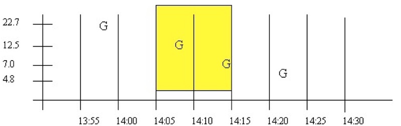
- Case 1: Good Data Samples Before and After the Interval Timestamp
This is the typical case when compression is not used. There are 2 good data quality raw points. With interpolation, calculate the slope and offset of this line and interpolate the value at the interval timestamp. The 14:10 interval has a sample at 14:08 and at 14:14.
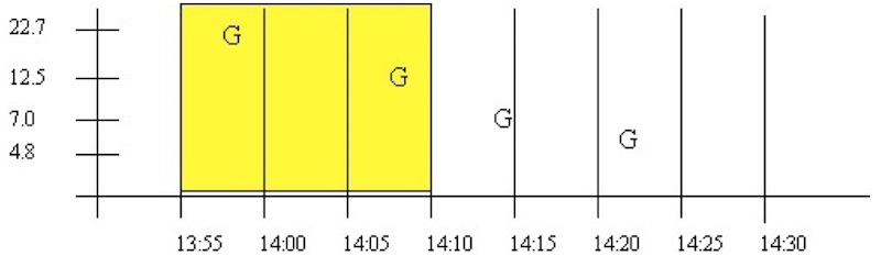
- Case 1a: Good Data Samples between the Interval Timestamp and the Start and End Time
In a similar case, there may be intervals with no raw samples, such as when data compression is used. Here, there is at least 1 good raw sample between the start time and interval, and at least 1 good raw sample between the interval and end time. The good raw samples are interpolated across intervals to determine values at the 14:00 and 14:05 intervals:
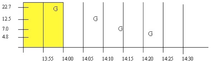
- Case 2: No Good Data between Start Time and Interval Timestamp
If no or bad data occurs before the interval, then the interval is given a bad data quality. The 13:55 interval is an example of this. Note that bad data is treated identically to no data.
- Case 3: No Good Data between Interval Timestamp and End Time
If no or bad data occurs after the interval then the interval is given a good data quality, but the value is simply stretched instead of interpolated. The 14:25 interval is an example of this. Note that bad data is treated identically to no data. Good data quality is attributed to the 14:30 interval
Data Quality
Unlike CurrentValue, RawByTime, and RawByNumber, Interpolated data does not assign an individual data quality to each returned sample. Since Interpolated, Lab, and Calculated retrieval modes can contain multiple samples in an interval, the data qualities of each point are combined and summarized as a percent good value.
Interpolated and Lab sampling determine the percent good using the same procedure, resulting in a value of either 100 or 0 (though the determined value may be different for each mode even with the same data). Intermediate percent good values are determined only for Calculated retrieval modes.
The following examples illustrate interpolated and lab sampling modes. For each example, you can see that the behavior is the same for lab and interpolated sampling by changing samplingmode=Interpolated to samplingmode=lab.
Example: Interpolated and Lab retrieval resulting in percent good of 100
This example illustrates the effect of bad data quality samples on the percent good statistic for an interval. The start and end times vary so that bad samples are included or excluded, which affects the percent good statistic
The data for BADDQTAG can be plotted as follows. The G is used to indicate a good data quality raw sample and the B indicates a sample of bad data quality. A query of the whole data set is shown.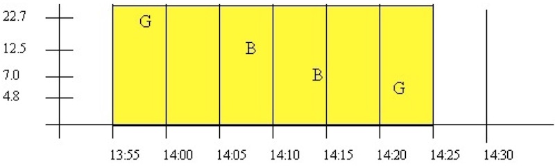
Using this query for a period starting with good data quality:
select timestamp, value, quality from ihrawdata where samplingmode=interpolated and timestamp >=
'29-Mar-2002 13:55' and timestamp <= '29-Mar-2002 14:25' and tagname  = baddqtag and numberofsamples = 1
This results in the following data quality:
| Timestamp | Value | Quality |
|---|---|---|
| 29-Mar-200214:25:00.000 | 4.80 | 100.00 |
The percent good is 100. Even though the interval contains bad data quality samples, the interval does not end with bad data quality. Percent good is determined this way because the purpose of interpolation and lab sampling is to determine the value and quality at the interval timestamp. On the other hand, Calculation modes operate on the full set of raw samples within an interval and therefore result in percent good values between 0 and 100.
This interval from 14:10 to 14:25 starts with a bad data quality sample but ends with a good sample, so the results are the same. That is, the query:
select timestamp, value, quality from ihrawdata where samplingmode=interpolated and timestamp >=
 '29-Mar-2002 14:10' and timestamp <= '29-Mar-2002 14:25' and tagname  = baddqtag and numberofsamples = 1
produces the same percent good result of 100.
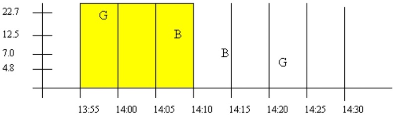
Example: Interpolated and Lab retrieval resulting in percent good of 0
This example shows some data patterns that result in a percent good of 0. An interval ending with a bad data quality sample, always results in a percent good of 0 for the interval.
| Timestsmp | Value | Quality |
|---|---|---|
| 29-Mar-2002 14:10:00.000 | 0.00 | 0.00 |
select timestamp, value, quality from ihrawdata where samplingmode=interpolated and timestamp >=
'29-Mar-2002 13:55' and timestamp <= '29-Mar-2002 14:10' and tagname = baddqtag and numberofsamples = 1| Timestamp | Value | Quality |
|---|---|---|
| 29-Mar-2002 14:10:00.000 | 0.00 | 0.00 |
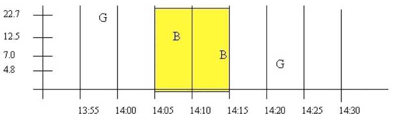
Example: Interpolated and Lab retrieval of an empty interval
The data quality of an empty interval depends on the previous and following raw samples. Intervals with a prior good data quality sample have a percent good of 100 and intervals preceded by a bad data quality sample (or no sample) have in a percent good of zero.
This query results in a percent good of 100:
select timestamp, value, quality from ihrawdata where samplingmode=interpolated and timestamp >=
 '29-Mar-2002 14:00' and timestamp <= '29-Mar-2002 14:05' and tagname  = baddqtag and numberofsamples = 1
Both of these queries produce a percent good of 0. The first has no preceding sample and the second is preceded by bad data:
select timestamp, value, quality from ihrawdata where samplingmode=interpolated and timestamp >=
'29-Mar-2002 13:50' and timestamp <= '29-Mar-2002 13:55' and tagname  = baddqtag and numberofsamples = 1
select timestamp, value, quality from ihrawdata where samplingmode=interpolated and timestamp >=
'29-Mar-2002 14:15' and timestamp <= '29-Mar-2002 14:20' and tagname  = baddqtag and numberofsamples = 1
The lab retrieval at 14:15 has a value of 7 but quality of 0. Note that you should almost always ignore specific values when the percent good is 0.