Using the Time Series Service

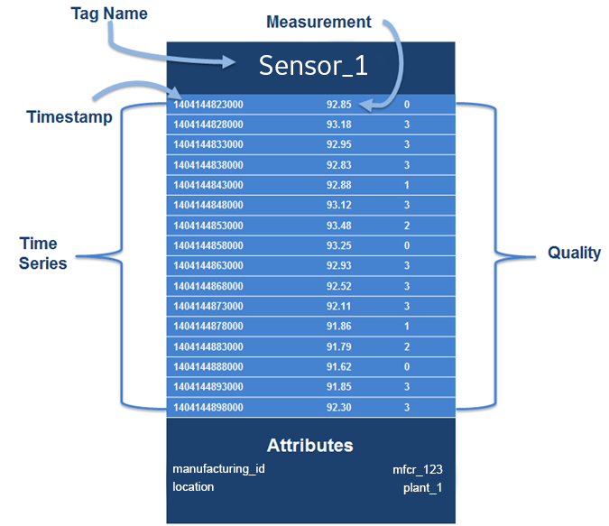
Time Series Data Model

A time series uses tags, which are often used to represent sensors (for example, a temperature sensor).

Data Ingestion

Time series data sets are based on the idea of tags, which represent different types of values measured by sensors (for example, temperature or pressure). A data record consists of one Tag Name (Sensor type), and multiple datapoints, each comprised of a Timestamp (Time) and a Measurement (Value). As additional options, each datapoint can also contain the quality of its data, and the overall record can contain multiple attributes (key/value pairs) describing the asset.

Table 1. Time Series Data Model Structure
Term	Definition
Tag name	(Required) Name of the tag (for example, "Temperature"). This does not need to be a unique value, and typically numerous sensors representing the same tag type will share this same tag name. Do not use the tag name to store attributes; you should instead store attributes like the sensor ID in the Attributes section. The tag name can contain alphanumeric characters, periods (.), slashes (/), dashes (-), underscores (_) and spaces and is limited to a maximum 256 characters.
Timestamp	(Required) The date and time in UNIX epoch time, with millisecond precision.
Measurement	(Required) The value produced from your sensor. See Data Types for more information on what is accepted. Do not include the unit of measurement in the field, for example, `98'C` ).
Qualities	(Optional) Quality of the data, represented by the values 0, 1, 2, 3. See Data Quality below for an explanation of data quality values.
Attribute	(Optional) Attributes are key/value pairs used to store data associated with a tag (for example: "ManufacturerGE":"AircraftID230"). This is useful for filtering data. Note: Attributes allow you to store additional relevant details about that specific data point???they should not be used to store large amounts of data. Do not use null values.
BackFill	(Optional) BackFill is a boolean flag that can be used to indicate whether this ingestion request includes backFill or non-live data. Data ingested with this option enabled will not be available to query immediately, but will be available eventually. Example: backFill: true Note: "backFill" field is a boolean and setting it to any other data type would return 400 (Bad Request).

Data Quality

You can tag data with values that represent data quality, which enables you to query by quality in cases where you want to retrieve or process only data of a specific level of quality. Using data quality can help to ensure that the data you get back in the query result is the most relevant for your purpose.


Value	Description
0	Bad quality.
1	Uncertain quality.
2	Not applicable.
3	Good quality. If you do not specify quality, the default is good (3).

Data Types

The Time Series ingestion service accepts mixed data types.

The following table shows sample input and output for mixed variable types (text, number, and null). When designing your data model:

Do not use attributes as tag names. Keep the tag name as the type of data produced by the sensor (for example, "Temperature" or "Pressure"), and use attributes to distinguish between distinct sensors.
Do not use timestamps as measurement values in your application.


Ingestion JSON Input	Ingestion JSON Input Type	Query Output	Datapoint Type
27	long	27	number
"34"	string (max 256 characters)	34	number
3.345	float	3.345	number
"1.123"	string (max 256 characters)	1.123	number
"1.0E-2"	string (256 characters)	0.01	number
"abc"	string (max 256 characters)	"abc"	text
"true"	string (max 256 characters)	"true"	text
true / false	boolean	"true" / "false"	text
"null"	string (max 256 characters)	"null"	text
null	null	null	Null
""	string (max 256 characters)	""	null
" "	string (max 256 characters)	" "	null

Data Consumption

The Time Series service provides REST APIs for querying and aggregating time series data. The API allows you to:

Query time series data specifying tags (sensors, etc) and a time window.
Filter by attribute values.
Retrieve all tags and attribute keys from the time series database.
Add aggregates and interpolate data points in a given time window.
Query the time series database for the latest values.
Note: When you use the GET latest API, the query returns the latest data point.
Delete tags and all the associated data points.

For more information about these APIs, see the API Documentation.

Ingesting Time Series Data

The Time Series service ingests data using the WebSocket protocol. You may use the Java client library to facilitate ingestion and to avoid setting up a WebSocket, or create your own Websocket connection if you prefer to use a language other than Java.

Ingest with the Java Client Library

After setting up your client, you may create Ingestion Requests using the Ingestion Request Builder. The following shows an example data ingestion request using the Java client. Library.

IngestionRequestBuilder ingestionBuilder = IngestionRequestBuilder.createIngestionRequest()
        .withMessageId("<MessageID>")
        .addIngestionTag(IngestionTag.Builder.createIngestionTag()
            .withTagName("TagName")
            .addDataPoints(
                Arrays.asList(
                            new DataPoint(new Date().getTime(),Math.random(), Quality.GOOD),
                            new DataPoint(new Date().getTime(), "BadValue", Quality.BAD),
                            new DataPoint(new Date().getTime(), null,Quality.UNCERTAIN))
                        )
            .addAttribute("AttributeKey", "AttributeValue")
            .addAttribute("AttributeKey2", "AttributeValue2")
            .build());

String json = ingestionBuilder.build().get(0); 
IngestionResponse response = ClientFactory.ingestionClientForTenant(tenant).ingest(json);
String responseStr = response.getMessageId() + response.getStatusCode();

Ingest with your own WebSocket Connection

You may also setup your own WebSocket in whatever language you prefer. It is recommended you find a WebSocket library in the language you are using to facilitate this process. Once you have a WebSocket library connected, point the request to the endpoint wss://<ingestion_url>. You must also provide the following headers:

Authorization: Bearer <token from UAA>
Predix-Zone-Id: <your zone id>
Origin: http://<your IP address or ???localhost???>

An example of a WebSocket implementation for Time Series ingestion is available at

https://github.com/PredixDev/timeseries-bootstrap/blob/master/src/main/java/com/ge/predix/solsvc/timeseries/bootstrap/client/TimeseriesClientImpl.java

Note: The ingestion URI and <Predix-Zone-Id> are included with the environment variables for your application when you bind your application to your Time Series service instance. To view the environment variables, on a command line, enter:

cf env <application_name>

Example Data Ingestion Request

The following shows an example of the JSON payload for an ingestion request:

URL: wss://ingestion_url
Headers:
   Authorization: Bearer <token from trusted issuer>
   Predix-Zone-Id: <Predix-Zone-Id>
   Origin: http://<origin-hostname>/
    
  
Request Payload:
{  
   "messageId": "<MessageID>",
   "body":[  
      {  
         "name":"<TagName>",
         "datapoints":[  
            [  
               <EpochInMs>,
               <Measure>,
               <Quality>
            ]
         ],
         "attributes":{  
            "<AttributeKey>":"<AttributeValue>",
            "<AttributeKey2>":"<AttributeValue2>"
         }
      }
   ]
}

Ingesting backFill data

When ingesting historical or non-live data, it is recommended to use the backFill option to avoid overloading the live data stream. Data ingested using this option will not be available to query immediately.

Note: This feature is not yet supported in the Java client.

The following JSON is an example of how to use the backFill option.

URL: wss://ingestion_url
Headers:
   Authorization: Bearer <token from trusted issuer>
   Predix-Zone-Id: <Predix-Zone-Id>
   Origin: http://<origin-hostname>/
    
  
Request Payload:
{  
   "messageId": "<MessageID>",
   "body":[  
      {  
         "name":"<TagName>",
         "datapoints":[  
            [  
               <EpochInMs>,
               <Measure>,
               <Quality>
            ]
         ],
         "attributes":{  
            "<AttributeKey>":"<AttributeValue>",
            "<AttributeKey2>":"<AttributeValue2>"
         }
      }
   ],
   "backFill": true
}

Ingestion Nuances

Consider the following when creating an ingestion request:

In previous releases, quality was supported as an attribute, but starting with this release,you must explicitly provide quality in each datapoint, along with the timestamp and measurement
The Time Series service now accepts compressed (GZIP) JSON payloads. The size limit for the actual JSON payload is 512 KB regardless of the ingestion request format. For compressed payloads, this means that the decompressed payload cannot exceed 512 KB.
The <Message Id> can be a string or integer, and must be unique. When using an integer the <MessageID> should be between 0 and 2⁶⁴ (18446744073709551616).
The <BackFill> must be a boolean. The ingestion request will return a 400 (Bad Request) status code if the <BackFill> is sent as any other data type. This is an optional parameter, and its value will be false if not specified.

Acknowledgement Message

An acknowledgement message is sent back to the client for each message packet. The following example shows an acknowledgement message:

{
        "messageId": <MessageID>,
        "statusCode": <AcknowledgementStatusCode>
}

The acknowledgement status codes are:


Code	Message
202	Accepted successfully
400	Bad request
401	Unauthorized
413	Request entity too large Note: The payload cannot exceed512KB.
503	Failed to ingest data

Tips for Data Ingestion

Spread ingestion requests over multiple connections, as sending numerous payloads over the same connection increases wait time for data availability over the query service. Also, be aware of our data plan when using multiple connections.

Pushing Time Series Data

Use the command-line interface as a simple way to interact with the Time Series service gateway. The time series gateway uses the WebSocket protocol for streaming ingestion. The ingestion endpoint format is: wss://ingestion_url.

The Web Socket protocol is used rather than HTTP because it can ingest a higher volume of data, which increases performance.

You can see an example of a WebSocket implementation for time series ingestion at https://github.com/predixdev/timeseries-bootstrap.

Note: The ingestion URI and <Predix-Zone-Id> are included with the environment variables for your application when you bind your application to your time series service instance. To view the environment variables, on a command line, enter:

cf env <application_name>

For all ingestion requests, use the token you received from UAA in the Authorization: section of the HTTP Header in the form of Bearer <token from trusted issuer>.

Note: In previous releases, quality was supported as an attribute, but starting with this release, you must explicitly provide quality in each datapoint, along with the timestamp and measurement.

Example Data Ingestion Request

The following shows an example of the JSON payload for an ingestion request:

URL: wss://ingestion_url
Headers:
   Authorization: Bearer <token from trusted issuer>
   Predix-Zone-Id: <Predix-Zone-Id>
   Origin: http://<origin-hostname>/
    
  
Request Payload:
{  
   "messageId": "<MessageID>",
   "body":[  
      {  
         "name":"<TagName>",
         "datapoints":[  
            [  
               <EpochInMs>,
               <Measure>,
               <Quality>
            ]
         ],
         "attributes":{  
            "<AttributeKey>":"<AttributeValue>",
            "<AttributeKey2>":"<AttributeValue2>"
         }
      }
   ]
}

The following shows an example of the JSON payload for an ingestion request to send it in backFill mode.

URL: wss://ingestion_url
Headers:
   Authorization: Bearer <token from trusted issuer>
   Predix-Zone-Id: <Predix-Zone-Id>
   Origin: http://<origin-hostname>/
    
  
{  
   "messageId": "<MessageID>",
   "body":[  
      {  
         "name":"<TagName>",
         "datapoints":[  
            [  
               <EpochInMs>,
               <Measure>,
               <Quality>
            ]
         ],
         "attributes":{  
            "<AttributeKey>":"<AttributeValue>",
            "<AttributeKey2>":"<AttributeValue2>"
         }
      }
   ],
   "backFill": true
}

The following shows an example data ingestion request if you are using a Java client.

IngestionRequestBuilder ingestionBuilder = IngestionRequestBuilder.createIngestionRequest()
        .withMessageId("<MessageID>")
        .addIngestionTag(IngestionTag.Builder.createIngestionTag()
                .withTagName("TagName")
                .addDataPoints(
                        Arrays.asList(
                                new DataPoint(new Date().getTime(), Math.random(), Quality.GOOD),
                                new DataPoint(new Date().getTime(), "Bad Value", Quality.BAD),
                                new DataPoint(new Date().getTime(), null, Quality.UNCERTAIN)
                        )
                )
                .addAttribute("AttributeKey", "AttributeValue")
                .addAttribute("AttributeKey2", "AttributeValue2")
                .build());

String json = ingestionBuilder.build().get(0);
IngestionResponse response = ClientFactory.ingestionClientForTenant(tenant).ingest(json);
String responseStr = response.getMessageId() + response.getStatusCode();

Note: The <MessageID> can be a string or integer, and must be unique. When using an integer the <MessageID> should be between 0 and 2⁶⁴ (18446744073709551616).

Note: <BackFill> must be a boolean value. A 400 ( Bad Request ) status code will be returned if <BackFill> is set as any other data type.

See tss-using-service.html#concept_dc613f2c-bb63-4287-9c95-8aaf2c1ca6f7 for more information about the structure of a time series tag.

Acknowledgement Message

An acknowledgement message is sent back to the client for each message packet. The following example shows an acknowledgement message:

{
    "messageId": <MessageID>,
    "statusCode": <AcknowledgementStatusCode>
}

Acknowledgement status codes include:


Code	Message
202	Accepted successfully
400	Bad request
401	Unauthorized
413	Request entity too large Note: The payload cannot exceed 512KB.
503	Failed to ingest data

Data Types

The Time Series ingestion service accepts mixed data types.

The following table shows sample input and output for mixed variable types (text, number, and null).


Ingestion JSON Input	Ingestion JSON Input Type	Query Output	Datapoint Type
27	long	27	number
???34???	string (max 256 characters)	34	number
3.345	float	3.345	number
???1.123???	string (max 256 characters)	1.123	number
???1.0E-2???	string (256 characters)	0.01	number
???abc???	string (max 256 characters)	???abc???	text
???true???	string (max 256 characters)	???true???	text
true / false	boolean	???true??? / ???false???	text
???null???	string (max 256 characters)	???null???	text
null	null	null	null
""	string (max 256 characters)	""	null
" "	string (max 256 characters)	" "	null

Querying Time Series Data

Before You Begin

Before you begin, perform all of the tasks in Setting Up and Configuring the Time Series Service.

About This Task

You can create queries using either the Java Client Library or via HTTP requests to the REST API. The API allows you to:

Query time series data specifying by tags (sensors, etc) and a time window.
Filter by attribute values.
Add aggregates and interpolate data points in a given time window.
Query the time series database for the latest values.

Only the synchronous API allows you to retrieve all tags and attribute keys from the time series database.

Procedure

View the environment variables for your application by entering the following on a command line:
```
cf env <application_name>
```
The query URI, trusted issuer token, and <Predix-Zone-Id> are included with the environment variables for your application. You will use this information in the HTTP header of your query.
Create your query.
The header for your query must be in the following format:
```
URL: https://query_url/v1/datapoints 
Method: POST
Headers:
    Authorization: Bearer <token from trusted issuer>
    Predix-Zone-Id: <Predix-Zone-Id>
```
Note: You can use both the GET and POST methods to query time series data. See tss-using-service.html#concept_0288d2ea-c99c-4148-b58a-a3ead6b78ef5 for more information about how to form a query request.

Tips for Time Series Data Queries

Attributes

Attributes should not contain high cardinality values for either the attribute key or value.
Do not store counters as attributes, as it degrades query performance.

GET vs POST Methods

Use the GET method for less complex queries. Responses can be cached in proxy servers and browsers.
Use the POST method as a convenience method when the query JSON is very long, and you do not need the request to be cached.
Note: The GET latest API returns the latest data point.

When using the POST API, the following rules apply:

Filters are the only supported operation, and they are optional.
Specifying a start time is optional, however, if you specify a start time, you must also specify an end time.
If you do not define a time window, the query retrieves the latest data points from the current time (now).

Performance

Multiple queries with fewer tags in each query leads to better performance than fewer queries that include more tags.

Data Points Limit

Data points in the query result cannot exceed the maximum limit of 500,000.

Time Series Query Optimization

To optimize query response times and service performance, keep the following recommendations and best practices in mind.

When deciding which tags to use for your data, keep in mind that tags are the primary means to ingest and query data in Time Series. Because Time Series data is indexed by tags, queries based on tags run much faster than attribute-based queries. For optimum performance, it is best to use tags to track data that you need to frequently query.
For example, to query data from California, New York, and Texas locations separately, you might create three queries. If you define an asset1 tag with a state attribute and query by attribute, run time can be slow. To optimize query performance, you can instead define a distinct tag for each query, for example, asset1_CA, asset1_NY, and asset1_TX.
Be aware that querying without using filters returns results faster. To minimize the time cost of query processing, it is best to avoid filtering to the greatest extent possible. For example, to find the latest data point, avoid using filters in your query.
To obtain the best performance, query by tags rather than by attributes. Tags are indexed, which speeds response time.
For fastest processing, specify the shortest time intervals that are useful to retrieve the data you need. For example, to find only one data point, set a one-month time window. Six queries with one-month time windows will run faster than a single query with a six-month time window.

Query Properties and Examples

Query Properties

Your query must specify a start field, which can be either absolute or relative. The end field is optional, and can be either absolute or relative. And you do not specify the end time, the query uses the current date and time.

Absolute start time ??? Expressed as an integer timestamp value in milliseconds.
Relative start time ??? Calculated relative to the current time. For example, if the start time is 15 minutes, the query returns all matching data points for the last 15 minutes. The relative start time is expressed as a string with the format <value><time-unit>-ago, where:
- <value> must be an integer greater than zero (0).
- <time-unit> ??? must be represented as follows:
  Time Unit Represents
  ms milliseconds
  s seconds
  mi minutes
  h hours
  d days
  w weeks
  mm months
  y years

Time Unit	Represents
ms	milliseconds
s	seconds
mi	minutes
h	hours
d	days
w	weeks
mm	months
y	years

Example General Query

You can use the time series APIs to list tags and attributes, as well as to query data points. You can query data points using start time, end time, tag names, time range, measurement, and attributes.

Note: The input JSON for an asynchronous query request is the same format as a synchronous query request. The header format is different, depending up which query API (asynchronous or synchronous) you specify in the URL. For more information, see tss-using-service.html#task_2cea3ed0-1f3a-48cb-8d55-42f037543941.

The following example shows a synchronous JSON data query with header using the POST method, with a limit of 1000 set for the number of data points to return in the query result:

URL: https://query_url/v1/datapoints 
Method: POST
Headers:
    Authorization: Bearer <token from trusted issuer>
    Predix-Zone-Id: <Predix-Zone-Id>
Payload:
{
?? ?? "start": 1427463525000,
?? ?? "end": 1427483525000,
?? ?? "tags": [
?? ?? ?? ??{
?? ?? ?? ?? ?? ?? "name": [
?? ?? ?? ?? ?? ?? ?? ?? "ALT_SENSOR",
?? ?? ?? ?? ?? ?? ?? ?? "TEMP_SENSOR"
?? ?? ?? ?? ?? ?? ],
?? ?? ?? ?? ?? ?? "limit": 1000,
?? ?? ?? ?? ?? ?? "aggregations": [
              {
?? ?? ?? ?? ?? ?? ?? ?? "type": "avg",
?? ?? ?? ?? ?? ?? ?? ?? "interval": "1h"
?? ?? ?? ?? ?? ?? ?? }
            ],
?? ?? ?? ?? ?? ?? "filters": {
?? ?? ?? ?? ?? ?? ?? ?? "attributes": {
?? ?? ?? ?? ?? ?? ?? ?? ?? ?? "host": "<host>",
?? ?? ?? ?? ?? ?? ?? ?? ?? ?? "type": "<type>"
?? ?? ?? ?? ?? ?? ?? ?? },
?? ?? ?? ?? ?? ?? ?? ?? "measurements": {
?? ?? ?? ?? ?? ?? ?? ?? ?? ?? "condition": "ge",
?? ?? ?? ?? ?? ?? ?? ?? ?? ?? "values": "23.1"
?? ?? ?? ?? ?? ?? ?? ?? },
?? ?? ?? ?? ?? ?? ?? ?? "qualities": {
?? ?? ?? ?? ?? ?? ?? ?? ?? ?? "values": [
?? ?? ?? ?? ?? ?? ?? ?? ?? ?? ?? ?? "0",
?? ?? ?? ?? ?? ?? ?? ?? ?? ?? ?? ?? "3"
?? ?? ?? ?? ?? ?? ?? ?? ?? ?? ]
?? ?? ?? ?? ?? ?? ?? ?? }
?? ?? ?? ?? ?? ?? },
?? ?? ?? ?? ?? ?? "groups": [
?? ?? ?? ?? ?? ?? ?? ?? {
?? ?? ?? ?? ?? ?? ?? ?? ?? ?? "name": "attribute",
?? ?? ?? ?? ?? ?? ?? ?? ?? ?? "attributes": [
?? ?? ?? ?? ?? ?? ?? ?? ?? ?? ?? ?? "attributename1",
?? ?? ?? ?? ?? ?? ?? ?? ?? ?? ?? ?? "attributename2"
?? ?? ?? ?? ?? ?? ?? ?? ?? ?? ]
?? ?? ?? ?? ?? ?? ?? ?? }
?? ?? ?? ?? ?? ?? ]
?? ?? ?? ?? }
?? ?? ]
}

The following example shows an asynchronous JSON data query with header using the POST method, with a limit of 1000 set for the number of data points to return in the query result. The same payload is passed, note the difference in the header URL.

URL: https://query_url/v1/datapoints/async 
Method: POST
Headers:
    Authorization: Bearer <token from trusted issuer>
    Predix-Zone-Id: <Predix-Zone-Id>
Payload:
{
?? ?? "start": 1427463525000,
?? ?? "end": 1427483525000,
?? ?? "tags": [
?? ?? ?? ??{
?? ?? ?? ?? ?? ?? "name": [
?? ?? ?? ?? ?? ?? ?? ?? "ALT_SENSOR",
?? ?? ?? ?? ?? ?? ?? ?? "TEMP_SENSOR"
?? ?? ?? ?? ?? ?? ],
?? ?? ?? ?? ?? ?? "limit": 1000,
?? ?? ?? ?? ?? ?? "aggregations": [
              {
?? ?? ?? ?? ?? ?? ?? ?? "type": "avg",
?? ?? ?? ?? ?? ?? ?? ?? "interval": "1h"
?? ?? ?? ?? ?? ?? ?? }
            ],
?? ?? ?? ?? ?? ?? "filters": {
?? ?? ?? ?? ?? ?? ?? ?? "attributes": {
?? ?? ?? ?? ?? ?? ?? ?? ?? ?? "host": "<host>",
?? ?? ?? ?? ?? ?? ?? ?? ?? ?? "type": "<type>"
?? ?? ?? ?? ?? ?? ?? ?? },
?? ?? ?? ?? ?? ?? ?? ?? "measurements": {
?? ?? ?? ?? ?? ?? ?? ?? ?? ?? "condition": "ge",
?? ?? ?? ?? ?? ?? ?? ?? ?? ?? "values": "23.1"
?? ?? ?? ?? ?? ?? ?? ?? },
?? ?? ?? ?? ?? ?? ?? ?? "qualities": {
?? ?? ?? ?? ?? ?? ?? ?? ?? ?? "values": [
?? ?? ?? ?? ?? ?? ?? ?? ?? ?? ?? ?? "0",
?? ?? ?? ?? ?? ?? ?? ?? ?? ?? ?? ?? "3"
?? ?? ?? ?? ?? ?? ?? ?? ?? ?? ]
?? ?? ?? ?? ?? ?? ?? ?? }
?? ?? ?? ?? ?? ?? },
?? ?? ?? ?? ?? ?? "groups": [
?? ?? ?? ?? ?? ?? ?? ?? {
?? ?? ?? ?? ?? ?? ?? ?? ?? ?? "name": "attribute",
?? ?? ?? ?? ?? ?? ?? ?? ?? ?? "attributes": [
?? ?? ?? ?? ?? ?? ?? ?? ?? ?? ?? ?? "attributename1",
?? ?? ?? ?? ?? ?? ?? ?? ?? ?? ?? ?? "attributename2"
?? ?? ?? ?? ?? ?? ?? ?? ?? ?? ]
?? ?? ?? ?? ?? ?? ?? ?? }
?? ?? ?? ?? ?? ?? ]
?? ?? ?? ?? }
?? ?? ]
}

The following is an example asynchronous query response.

{
    "statusCode": 202,
"correlationId": "00000166-36cc-b44b-5d85-db5918aeed67",
"expirationTime" : 1533666448748
}

The following shows an example of a query request if you are using the Java time series client library:

QueryBuilder builder = QueryBuilder.createQuery()
        .withStartAbs(1427463525000L)
        .withEndAbs(1427483525000L)
        .addTags(
                QueryTag.Builder.createQueryTag()
                        .withTagNames(Arrays.asList("ALT_SENSOR", "TEMP_SENSOR"))
                        .withLimit(1000)
                        .addAggregation(Aggregation.Builder.averageWithInterval(1, TimeUnit.HOURS))
                        .addFilters(FilterBuilder.getInstance()
                                .addAttributeFilter("host", Arrays.asList("<host>")).build())
                        .addFilters(FilterBuilder.getInstance()
                                .addAttributeFilter("type", Arrays.asList("<type>")).build())
                        .addFilters(FilterBuilder.getInstance()
                                .addMeasurementFilter(FilterBuilder.Condition.GREATER_THAN_OR_EQUALS, Arrays.asList("23.1")).build())
                        .addFilters(FilterBuilder.getInstance()
                                .withQualitiesFilter(Arrays.asList(Quality.BAD, Quality.GOOD)).build())
                        .build());
QueryResponse response = ClientFactory.queryClientForTenant(tenant).queryAll(builder.build());

Use the token you receive from the trusted issuer in the HTTP Header ???Authorization??? for all query requests in the form of 'Bearer <token from trusted issuer>'.

Note:

You can use both the GET and POST methods to query time series data. Use the query API with the GET HTTP method by passing the query JSON as a URL query parameter. The GET method allows requests and responses to be cached in proxy servers and browsers.

In cases where the query JSON is very long and exceeds query parameter length (for some browsers), use POST as an alternate method to query the time series API.

POST requests have no restrictions on data length. However, requests are never cached. The Time Series service API design supports complex, nested time series queries for multiple tags and their attributes. For example, more complex queries can include aggregations and filters.

For more information about this API, see the API Documentation.

Note: Tag names, measurement, and attributes are case-sensitive and can contain only alphanumeric characters, periods (.), slashes (/), dashes (-), and underscores (_).

Requesting Asynchronous Query Status

You can request the status of an asynchronous query only, this type of request is not supported for synchronous queries. The asynchronous status query request must be in the following format.

URL: http://query_uri/v1/datapoints/query/status
	Method: GET/POST
	Headers:
    	Authorization: Bearer <token from trusted issuer>
		Predix-Zone-Id: <Predix-Zone-Id>
             	Parameters:
		correlationID: <correlationID>
		jobStatusOnly: True

The jobStatusOnly field is not required. The jobStatusOnly parameter will default to True if not provided.

The following is an example of an asynchronous query response.

HTTP Code: 200

{  
    "request":{  
      "correlationID":"aaa-aaa-aaa",
      "tenantID":"zzz-zzz-zzz",
      "operationType":"query"
   },
   "lastUpdated":12345678,
   "created":12345678,
   "status":"Completed",
   "statusText":"Successfully completed",
   "message":{  
   }
}

Requesting Asynchronous Query Results

The request for asynchronous query results must be in the following format.

URL: http://query_uri/v1/datapoints/query/status
	Method: GET/POST
	Headers:
    	Authorization: Bearer <token from trusted issuer>
		Predix-Zone-Id: <Predix-Zone-Id>
             	Parameters:
		correlationID: <correlationID>
		jobStatusOnly: False

The jobStatusOnly field is not required. The jobStatusOnly parameter will default to True if not provided. This field indicates if the status query response should contain the time series data (False) or only the requested job status (True).

The following example shows asynchronous query results.

HTTP Code: 200

{  
    "request":{  
      "correlationID":"aaa-aaa-aaa",
      "tenantID":"zzz-zzz-zzz",
      "operationType":"query"
   },
   "lastUpdated":12345678,
   "created":12345678,
   "statusText":"finished???,
   "message??? : ??????,
   "queryResults": 
      "{
         "tags": [{
            "name": "test.async",
            "results": [{
               "groups": [{
                  "name": "type",
                  "type": "number"
               }],
               "attributes": {},
               "values": [
                  [1435776300000, 28.875, 3]
               ]
            }],
            "stats": {
               "rawCount": 4
            }
         }]
      }"
}

Valid response for statusText can be one of the following.

created
paused
processing
finished
not found
expired
failed

If the query completes successfully, the queryResults field contains the JSON response from the query.

Using Relative Start and End Times in a Query

This example shows a JSON query using a relative start time, with a value of "15" and a unit of "minutes", and an absolute end time in milliseconds.

{
?? ?? "start": "15mi-ago",
    "end": 1427483525000,
?? ?? "tags": [
?? ?? ?? ?? {
?? ?? ?? ?? ?? ?? "name": "ALT_SENSOR",
?? ?? ?? ?? ?? ?? "limit": 1000
?? ?? ?? ??}
?? ??]
}

This example shows a query using a relative start time using the time series client library:

QueryBuilder builder = QueryBuilder.createQuery()
        .withStartRelative(15, TimeUnit.MINUTES, TimeRelation.AGO)
        .withEndAbs(1427483525000L)
        .addTags(
                QueryTag.Builder.createQueryTag()
                        .withTagNames(Arrays.asList("ALT_SENSOR"))
                        .withLimit(1000)
                        .build());

QueryResponse queryResponse = ClientFactory.queryClientForTenant(tenant).queryAll(builder.build());

This example shows a JSON query using the absolute start time in milliseconds, and a relative end time with a value of "5" and a unit of "minutes".

{
?? ?? "start": 1427463525000,
?? ?? "end": "5mi-ago", 
?? ?? "tags": [
?? ?? ?? ?? {
?? ?? ?? ?? ?? ?? "name": "ALT_SENSOR",
?? ?? ?? ?? ?? ?? "limit": 1000
?? ?? ?? ??}
?? ??]
}

This example shows a query using an absolute start time and relative end time using the time series client library:

QueryBuilder builder = QueryBuilder.createQuery()
        .withStartAbs(1427463525000L)
        .withEndRelative(5, TimeUnit.MINUTES, TimeRelation.AGO)
        .addTags(
                QueryTag.Builder.createQueryTag()
                        .withTagNames(Arrays.asList("ALT_SENSOR"))
                        .withLimit(1000)
                        .build());

QueryResponse queryResponse = ClientFactory.queryClientForTenant(tenant).queryAll(builder.build());

Data Points Limit

The following limits apply to data queries:

Data points in the query result cannot exceed the maximum limit of 500,000.
Narrow your query criteria (for example, time window) to return a fewer number of data points.

Limiting the Data Points Returned by a Query

When you create a query, you can specify a limit for the number of data points returned in the query results. This example shows a JSON query with the "limit" property set to 1000.

{
?? ?? "start": 1427463525000,
?? ?? "end": 1427483525000,
?? ?? "tags": [
?? ?? ?? ?? {
?? ?? ?? ?? ?? ?? "name": "ALT_SENSOR",
?? ?? ?? ?? ?? ?? "limit": 1000
?? ?? ?? ??}
?? ??]
}

This example shows the same "limit" query using the time series client library.

QueryBuilder builder = QueryBuilder.createQuery()
        .withStartAbs(1427463525000L)
        .withEndAbs(1427483525000L)
        .addTags(
                QueryTag.Builder.createQueryTag()
                        .withTagNames(Arrays.asList("ALT_SENSOR"))
                        .withLimit(1000)
                        .build());

QueryResponse queryResponse = ClientFactory.queryClientForTenant(tenant).queryAll(builder.build());

Specifying the Order of Data Points Returned by a Query

The default order for query results is ascending, and it is ordered by timestamp. You can use the order property in your query request to specify the order in which you want the data points returned. This example returns the data points in descending order:

{
?? ?? "start": 1427463525000,
?? ?? "end": 1427483525000,
?? ?? "tags": [
?? ?? ?? ?? {
?? ?? ?? ?? ?? ?? "name": "ALT_SENSOR",
?? ?? ?? ?? ?? ?? "order": "desc"
?? ?? ?? ??}
?? ??]
}

This example shows the same "order" query using the time series client library:

QueryBuilder builder = QueryBuilder.createQuery()
        .withStartAbs(1427463525000L)
        .withEndAbs(1427483525000L)
        .addTags(
                QueryTag.Builder.createQueryTag()
                        .withTagNames(Arrays.asList("ALT_SENSOR"))
                        .withOrder(QueryTag.Order.DESCENDING)
                        .build());

QueryResponse queryResponse = ClientFactory.queryClientForTenant(tenant).queryAll(builder.build());

Query for Latest Data Point Example

The Time Series API provides both a GET and POST method for retrieving the most recent data point within the defined time window. By default, unless you specify a start time, the query goes back 15 days. When using the POST API, the following rules apply:

Filters are the only supported operation, and they are optional.
Specifying a start time is optional. However, if you do specify the start time, you must also specify an end time.
If you do not define a time window, the query retrieves the latest data points from the current time (now).

The following shows an example of a JSON query for the latest data point with no time window defined:

{
    "tags": [
        {
            "name": "ALT_SENSOR",
            "filters": {
                "measurements": {
                    "condition": "le",
                    "value": 10
                }
            }
        }
    ]
}

This example shows the same query using the time series client library:

QueryBuilder builder = QueryBuilder.createQuery()
        .addTags(
                QueryTag.Builder.createQueryTag()
                        .withTagNames(
                                Arrays.asList("ALT_SENSOR")
                        )
                        .addFilters(FilterBuilder.getInstance()
                            .addMeasurementFilter(FilterBuilder.Condition.LESS_THAN_OR_EQUALS, Arrays.asList("10"))
                                .build())
                        .build());
QueryResponse queryResponse = ClientFactory.queryClientForTenant(tenant).queryForLatest(builder.build());

Query for Data Points Relative to a Time Stamp Examples

You can query for data points relative to a given time stamp by passing the parameter "direction" and specifying whether you want results after ("forward") or before ("backward") that point. Use the "limit" filter to specify the number of data points to return.

Query for Data Points After a Given Time Stamp

This example shows how you can query for data points for results after ("forward") a given time stamp. This example shows a JSON ingestion data query.

[{
	"name": "test.forward.integer",
	"datapoints": [
		[1435776300000, 2, 3],
		[1435776400000, 10, 3],
		[1435776500000, 1, 3],
		[1435776550000, 2, 3],
		[1435776600000, 6, 3],
		[1435776700000, 2, 3],
		[1435776800000, 13, 3],
		[1435776900000, 3, 0]
	]
}]

This example shows a query using the parameter "direction" with the value "forward" with a given "start" time. The "limit" filter specifies "3" data points are to be returned.

{
	"start": 1435776550000,
	"direction": "forward",
        "tags": [{
		"name": "test.forward.integer",
	        "limit": 3
	}]
}

This example shows the results returned.

{
	"tags": [{
		"name": "test.forward.integer",
		"results": [{
			"values": [
                            [1435776550000, 2, 3],
		            [1435776600000, 6, 3],
		            [1435776700000, 2, 3]
			],		
                        "groups": [{
				"name": "type",
				"type": "number"
			}],
			"attributes": {}
		}],
		"stats": {
			"rawCount": 8
		}
	}]
}

Query for Data Points Before a Given Time Stamp

This example shows how you can query for data points for results before ("backward") a given time stamp. This example shows a JSON ingestion data query.

[{
	"name": "test.backward.integer",
	"datapoints": [
		[1435776300000, 2, 3],
		[1435776400000, 10, 3],
		[1435776500000, 1, 3],
		[1435776550000, 2, 3],
		[1435776600000, 6, 3],
		[1435776700000, 2, 3],
		[1435776800000, 13, 3],
		[1435776900000, 3, 0]
	]
}]

This example shows a query using the parameter "direction" with the value "backward" with a given "start" time. The "limit" filter specifies "3" data points are to be returned.

{
	"start": 1435776550000,
	"direction": "backward",
        "tags": [{
		"name": "test.backward.integer",
	        "limit": 3
	}]
}

This example shows the results returned.

{
	"tags": [{
		"name": "test.backward.integer",
		"results": [{
			"values": [
                            [1435776400000, 10, 3],
		            [1435776500000, 1, 3],
		            [1435776550000, 2, 3]
			],		
                        "groups": [{
				"name": "type",
				"type": "number"
			}],
			"attributes": {}
		}],
		"stats": {
			"rawCount": 8
		}
	}]
}

Data Aggregators

Aggregation functions allow you to perform mathematical operations on a number of data points to create a reduced number of data points. Aggregation functions each perform distinct mathematical operations and are performed on all the data points included in the sampling period.

Note: Data points that are string or null types within the time range are ignored in data aggregations and not returned in the response.

You can use the <query url>/v1/aggregations endpoint to get a list of the available aggregations.

For more information about these APIs, see the API Documentation.

Aggregations are processed in the order specified in the query. The output of an aggregation is passed to the input of the next until they are all processed.

Aggregator Parameters

The unit and sampling aggregators are common to more than one aggregator.

Unit is a string and must be one of the following:

MILLISECONDS
SECONDS
MINUTES
HOURS
DAYS
WEEKS

The sampling aggregator is a JSON object that contains a value (integer) and a unit.

Range Aggregator

You can set the following parameters on any range aggregator:

sampling ??? JSON object that contains a unit and value.
align_start_time (boolean) ??? Set to true if you want the time for the aggregated data point for each range to fall on the start of the range instead of being the value for the first data point within that range.
align_sampling (boolean) ??? Set to true if you want the aggregation range to be aligned based on the sampling size and you want the data to take the same shape, when graphed, as you refresh the data.
start_time (long) ??? Start time from which to calculate the ranges (start of the query).
time_zone (long time zone format) ??? Time zone to use for time-based calculations.

Aggregators


Name	Type	Parameters	Description
`avg`	Average	Extends the `range` aggregator.	Returns the average of the values.
`count`	Count	Extends the `range` aggregator.	Counts the number of data points.
`dev`	Standard Deviation	Extends the `range` aggregator.	Returns the standard deviation of the time series.
`diff`	Difference	Extends the `range` aggregator.	Calculates the difference between successive data points.
`div`	Divide	The `divisor` (double) parameter is required. This is the value by which to divide data points.	Returns each data point divided by the specified value of the `divisor` property.
`gaps`	Gaps	Extends the `range` aggregator.	Marks gaps in data with a null data point, according to the sampling rate.
`interpolate`	Interpolate	Extends the `range` aggregator.	Does linear interpolation for the chosen window.
`least_squares`	Least Squares	Extends the `range` aggregator.	Returns two points that represent the best fit line through the set of data points for the range.
`max`	Maximum	Extends the `range` aggregator.	Inherits from the `range` aggregator. Returns the most recent largest value.
`min`	Minimum	Extends the `range` aggregator.	Returns the most recent smallest value.
`percentile`	Percentile	Extends the `range` aggregator. `percentile` ??? Percentile to count.	Calculates a probability distribution, and returns the specified percentile for the distribution. The ???percentile??? value is defined as 0 < percentile <= 1 where .5 is 50% and 1 is 100%.
`rate`	Rate	`sampling` ??? Sets the sampling for calculating the rate. `unit` ??? Required. Set the sampling duration as MILLISECONDS, SECONDS, MINUTES, HOURS, DAYS, or WEEKS. For example, if you set the unit to HOUR, the sampling rate is over one hour. `time_zone` ??? Must use the long format, for example:	Returns the rate of change between a pair of data points.
`sampler`	Sampler	Optional parameters include: `unit` ??? Set the sampling duration as MILLISECONDS, SECONDS, MINUTES, HOURS, DAYS, or WEEKS. For example, if you set the unit to HOUR, the sampling rate is over one hour. `time_zone` ??? Must use the long format, for example:	Calculates the sampling rate of change for the data points.
`scale`	Scale	`factor` (double) ??? Scaling value.	Scales each data point by a factor.
`sum`	Sum	Extends the `range` aggregator.	Returns the sum of all values.
`trendmode`	Trend Mode	`sampling` ??? Sets the sampling for calculating the min and max within each interval.	Returns the `min` and `max` values within each interval. Note: Trend Mode converts all longs to double. This causes a loss of precision for very large long values.

Aggregation Examples

Data Interpolation

You can interpolate data between raw data samples when data is missing and query for results based on a time interval (for example, every one hour). The following shows a sample request for interpolating data for every hour for the given time window:

{  
   "start":1432667547000,
   "end":1432667552000,
   "tags":[  
      {  
         "name":"phosphate.level",
         "aggregations":[  
            {  
               "type":"interpolate",
               "interval": "1h"
            }
         ]
      }
   ]
}

Querying to Have a Specific Number of Data Points Returned

This shows an example of querying data using interpolation mode and specifying the time window and number of data points to return:

{  
   "start":1432667547000,
   "end":1432667552000,
   "tags":[  
      {  
         "name":"phosphate.level",
         "aggregations":[  
            {  
               "type":"interpolate",
               "sampling":{  
                  "datapoints":500
               }
            }
         ]
      }
   ]
}

Querying for the Average Value

This shows an example of querying for the average value with a 30-second interval on which to aggregate the data:

{
	"tags": [{
		"name": "Compressor-2015",
		"aggregations": [{
			"type": "avg",
			"sampling": {
				"unit": "s",
				"value": "30"
			}
		}]
	}],
	"start": 1452112200000,
	"end": 1453458896222
}

Querying for Values Between Boundaries

This shows an example of querying data using interpolation mode between "start", "end", "interval", and "extension" (24 hours or less/in milliseconds) parameter values. Predix Time Series will interpolate between start - extension and end + extension and return values between start + interval to end, inclusive.

Example Ingestion JSON

[{
	"name": "test.interpolation.extension.integer",
	"datapoints": [
		[1200, 3.0, 3],
		[2500, 4.0, 3],
		[3200, 2.0, 3],
	]
}]

Example Query

{
	"start": 1000,
	"end": 3000,
	"tags": [{
		"name": "test.interpolation.extension.integer",
		"aggregations": [{
			"type": "interpolate",
                        "interval": "1000ms", 
                        "extension": "1000"
                 }]
	}]
}

Example Result

{
  "tags": [
    {
      "name": "test.interpolation.extension.integer",
      "results": [
        {
          "groups": [
            {
              "name": "type", 
              "type": "number"
            }
          ],
          "values": [
            [2000, 3.6153846153846154, 3],
            [3000, 2.571428571428571, 3],
          ],
          "attributes": {}
        }
      ],
      "stats": {
        "rawCount": 3
      }
    }
  ]
}

Average With Mixed Data Types

The Average aggregator returns the average of the values.

Example Ingestion JSON

[{
	"name": "test.average.mixedType",
	"datapoints": [
		[1435776300000, 2, 1],
		[1435776400000, null],
		[1435776500000, 10.5, 3],
		[1435776550000, "100", 2],
		[1435776600000, "string"],
		[1435776700000, "string36"],
		[1435776800000, true],
		[1435776900000, 3, 0]
	]
}]

Example Query

{
	"start": 1435766300000,
	"end": 1435777000000,
	"tags": [{
		"name": "test.average.mixedType",
		"aggregations": [{
			"type": "avg",
			"sampling": {
				"datapoints": 1
			}
		}]
	}]
}

The following shows an example of the average aggregator using the time series client library:

QueryBuilder builder = QueryBuilder.createQuery()
        .withStartAbs(1432671129000L)
        .withEndAbs(1432672230500L)
        .addTags(
                QueryTag.Builder.createQueryTag()
                        .withTagNames(
                                Arrays.asList("ALT_SENSOR")
                        )
                        .addAggregation(Aggregation.Builder.averageWithInterval(3600, TimeUnit.SECONDS))
                        .build());
QueryResponse queryResponse = ClientFactory.queryClientForTenant(tenant).queryForLatest(builder.build());

Example Result

{
	"tags": [{
		"name": "test.average.mixedType",
		"results": [{
			"groups": [{
				"name": "type",
				"type": "number"
			}],
			"attributes": {},
			"values": [
				[1435776300000, 28.875, 3]
			]
		}],
		"stats": {
			"rawCount": 4
		}
	}]
}

Average With Double Data Types

The Average aggregator returns the average of the values.

Example Ingestion JSON

[{
	"name": "test.average.doubleType",
	"datapoints": [
		[1435766300000, 2.0],
		[1435766400000, 2.5],
		[1435766500000, 3.0],
		[1435766550000, 3.5],
		[1435766600000, 4.0],
		[1435766700000, 50.0],
		[1435766800000, 100.0],
		[1435766900000, 150.5],
		[1435777000000, 175.0],
		[1435777100000, 175.5],
		[1435777200000, 200.0],
		[1435777300000, 225.0],
		[1435777400000, 225.5],
		[1435777500000, 250],
		[1435777600000, 300.0]
	]
}]

Example Query

{
	"start": 1435766300000,
	"end": 1435787600000,
	"tags": [{
		"name": "test.average.doubleType",
		"aggregations": [{
			"type": "avg",
			"sampling": {
				"datapoints": 1
			}
		}]
	}]
}

Example Result

{
	"tags": [{
		"name": "test.average.doubleType",
		"results": [{
			"groups": [{
				"name": "type",
				"type": "number"
			}],
			"attributes": {},
			"values": [
				[1435766300000, 124.43333333333334, 3]
			]
		}],
		"stats": {
			"rawCount": 15
		}
	}]
}

Count With Mixed Data Types

The Count aggregator returns the most recent largest value.

Example 1

Example Ingestion JSON

[{
	"name": "test.count.mixedType",
	"datapoints": [
		[1435776300000, 2, 1],
		[1435776400000, null],
		[1435776500000, 10.5, 3],
		[1435776550000, "100", 2],
		[1435776600000, "string"],
		[1435776700000, "string36"],
		[1435776800000, true],
		[1435776900000, 3, 0]
	]
}]

Example Query

{
	"start": 1435766300000,
	"end": 1435777000000,
	"tags": [{
		"name": "test.count.mixedType",
		"filters": {
			"qualities": {
				"values": ["3"]
			}
		},
		"aggregations": [{
			"type": "trendmode",
			"sampling": {
				"datapoints": 1
			}
		}, {
			"type": "count",
			"sampling": {
				"datapoints": 1
			}
		}]
	}]
}

Example Result

{
	"tags": [{
		"name": "test.count.mixedType",
		"results": [{
			"groups": [{
				"name": "type",
				"type": "number"
			}],
			"filters": {
				"qualities": {
					"values": ["3"]
				}
			},
			"attributes": {},
			"values": [
				[1435776500000, 1, 3]
			]
		}],
		"stats": {
			"rawCount": 1
		}
	}]
}

Example 2

Example Ingestion JSON

[{
	"name": "test.count.mixedType",
	"datapoints": [
		[1435776300000, 2, 1],
		[1435776400000, null],
		[1435776500000, 10.5, 3],
		[1435776550000, "100", 2],
		[1435776600000, "string"],
		[1435776700000, "string36"],
		[1435776800000, true],
		[1435776900000, 3, 0]
	]
}]

Example Query

{
	"start": 1435766300000,
	"end": 1435777000000,
	"tags": [{
		"name": "test.count.mixedType",
		"aggregations": [{
			"type": "trendmode",
			"sampling": {
				"datapoints": 1
			}
		}, {
			"type": "count",
			"sampling": {
				"datapoints": 1
			}
		}]
	}]
}

Example Result

{
	"tags": [{
		"name": "test.count.mixedType",
		"results": [{
			"groups": [{
				"name": "type",
				"type": "number"
			}],
			"attributes": {},
			"values": [
				[1435776300000, 2, 3]
			]
		}],
		"stats": {
			"rawCount": 4
		}
	}]
}

Example 3

Example Ingestion JSON

[{
	"name": "test.count.mixedType",
	"datapoints": [
		[1435776300000, 2, 1],
		[1435776400000, null],
		[1435776500000, 10.5, 3],
		[1435776550000, "100", 2],
		[1435776600000, "string"],
		[1435776700000, "string36"],
		[1435776800000, true],
		[1435776900000, 3, 0]
	]
}]

Example Query

{
	"start": 1435766300000,
	"end": 1435777000000,
	"tags": [{
		"name": "test.count.mixedType",
		"aggregations": [{
			"type": "count",
			"sampling": {
				"datapoints": 1
			}
		}]
	}]
}

Example Result

{
	"tags": [{
		"name": "test.count.mixedType",
		"results": [{
			"groups": [{
				"name": "type",
				"type": "number"
			}],
			"attributes": {},
			"values": [
				[1435776300000, 4, 3]
			]
		}],
		"stats": {
			"rawCount": 4
		}
	}]
}

Count With Double Data Types

The Count aggregator returns the most recent largest value.

Example Ingestion JSON

[{
	"name": "test.count.mode.doubleType",
	"datapoints": [
		[1435766300000, 2.0],
		[1435766400000, 2.5],
		[1435766500000, 3.0],
		[1435766550000, 3.5, 2],
		[1435766600000, 4.0],
		[1435766700000, 50.0],
		[1435766800000, 100.0],
		[1435766900000, 150.5],
		[1435777000000, 175.0],
		[1435777100000, 175.5],
		[1435777200000, 200.0],
		[1435777300000, 225.0],
		[1435777400000, 225.5],
		[1435777500000, 250],
		[1435777600000, 300.0]
	]
}]

Example Query

{
	"start": 1435766300000,
	"end": 1435787600000,
	"tags": [{
		"name": "test.count.mode.doubleType",
		"aggregations": [{
			"type": "count",
			"sampling": {
				"datapoints": 1
			}
		}]
	}]
}

Example Result

{
	"tags": [{
		"name": "test.count.mode.doubleType",
		"results": [{
			"groups": [{
				"name": "type",
				"type": "number"
			}],
			"attributes": {},
			"values": [
				[1435766300000, 15, 3]
			]
		}],
		"stats": {
			"rawCount": 15
		}
	}]
}

Difference With Mixed Data Types

The Difference aggregator calculates the difference between successive data points.

Example Ingestion JSON

[{
	"name": "test.diff.mixedType",
	"datapoints": [
		[1435776300000, 2, 1],
		[1435776400000, null],
		[1435776500000, 10.5, 3],
		[1435776550000, "100", 2],
		[1435776600000, "string"],
		[1435776700000, "string36"],
		[1435776800000, true],
		[1435776900000, 3, 0]
	]
}]

Example Query

{
	"start": 1435766300000,
	"end": 1435777000000,
	"tags": [{
		"name": "test.diff.mixedType",
		"aggregations": [{
			"type": "diff"
		}]
	}]
}

Example Result

{
	"tags": [{
		"name": "test.diff.mixedType",
		"results": [{
			"groups": [{
				"name": "type",
				"type": "number"
			}],
			"attributes": {},
			"values": [
				[1435776500000, 8.5, 3],
				[1435776550000, 89.5, 3],
				[1435776900000, -97, 3]
			]
		}],
		"stats": {
			"rawCount": 4
		}
	}]
}

Divide With Mixed Data Types

The Divide aggregator returns each data point divided by the specified value of the divisor property.

Example Ingestion JSON

[{
	"name": "test.div.mixedType",
	"datapoints": [
		[1435776300000, 2, 1],
		[1435776400000, null],
		[1435776500000, 10.5, 3],
		[1435776550000, "100", 2],
		[1435776600000, "string"],
		[1435776700000, "string36"],
		[1435776800000, true],
		[1435776900000, 3, 0]
	]
}]

Example Query

{
	"start": 1435766300000,
	"end": 1435777000000,
	"tags": [{
		"name": "test.div.mixedType",
		"aggregations": [{
			"type": "div",
			"divisor": 3
		}]
	}]
}

Example Result

{
	"tags": [{
		"name": "test.div.mixedType",
		"results": [{
			"groups": [{
				"name": "type",
				"type": "number"
			}],
			"attributes": {},
			"values": [
				[1435776300000, 0.6666666666666666, 3],
				[1435776500000, 3.5, 3],
				[1435776550000, 33.333333333333336, 3],
				[1435776900000, 1, 3]
			]
		}],
		"stats": {
			"rawCount": 4
		}
	}]
}

Divide With Double Data Types

The Divide aggregator returns each data point divided by the specified value of the divisor property.

Example Ingestion JSON

[{
	"name": "test.div.doubleType",
	"datapoints": [
		[1435766300000, 2.0],
		[1435766400000, 2.5],
		[1435766500000, 3.0],
		[1435766550000, 3.5],
		[1435766600000, 4.0],
		[1435766700000, 50.0],
		[1435766800000, 100.0],
		[1435766900000, 150.5],
		[1435777000000, 175.0],
		[1435777100000, 175.5],
		[1435777200000, 200.0],
		[1435777300000, 225.0],
		[1435777400000, 225.5],
		[1435777500000, 250],
		[1435777600000, 300.0]
	]
}]

Example Query

{
	"start": 1435766300000,
	"end": 1435787600000,
	"tags": [{
		"name": "test.div.doubleType",
		"aggregations": [{
			"type": "div",
			"divisor": 3
		}]
	}]
}

Example Result

{
	"tags": [{
		"name": "test.div.doubleType",
		"results": [{
			"groups": [{
				"name": "type",
				"type": "number"
			}],
			"attributes": {},
			"values": [
				[1435766300000, 0.6666666666666666, 3],
				[1435766400000, 0.8333333333333334, 3],
				[1435766500000, 1, 3],
				[1435766550000, 1.1666666666666667, 3],
				[1435766600000, 1.3333333333333333, 3],
				[1435766700000, 16.666666666666668, 3],
				[1435766800000, 33.333333333333336, 3],
				[1435766900000, 50.166666666666664, 3],
				[1435777000000, 58.333333333333336, 3],
				[1435777100000, 58.5, 3],
				[1435777200000, 66.66666666666667, 3],
				[1435777300000, 75, 3],
				[1435777400000, 75.16666666666667, 3],
				[1435777500000, 83.33333333333333, 3],
				[1435777600000, 100, 3]
			]
		}],
		"stats": {
			"rawCount": 15
		}
	}]
}

Gaps With Mixed Data Types

The Gaps aggregator marks gaps in data with a null data point, according to the sampling rate.

Example Ingestion JSON

[{
	"name": "test.gaps.mixedType",
	"datapoints": [
		[1435776300000, 2, 1],
		[1435776400000, null],
		[1435776500000, 10.5, 3],
		[1435776550000, "100", 2],
		[1435776600000, "string"],
		[1435776700000, "string36"],
		[1435776800000, true],
		[1435776900000, 3, 0]
	]
}]

Example Query

{
	"start": 1435766300000,
	"end": 1435777000000,
	"tags": [{
		"name": "test.gaps.mixedType",
		"aggregations": [{
			"type": "gaps",
			"interval": "100000ms"
		}]
	}]
}

Example Result

{
	"tags": [{
		"name": "test.gaps.mixedType",
		"results": [{
			"groups": [{
				"name": "type",
				"type": "number"
			}],
			"attributes": {},
			"values": [
				[1435776300000, 2, 1],
				[1435776400000, null, 3],
				[1435776500000, 10.5, 3],
				[1435776550000, 100, 2],
				[1435776600000, null, 3],
				[1435776700000, null, 3],
				[1435776800000, null, 3],
				[1435776900000, 3, 0]
			]
		}],
		"stats": {
			"rawCount": 4
		}
	}]
}

Gaps With Double Data Types

The Gaps aggregator marks gaps in data with a null data point, according to the sampling rate.

Example Ingestion JSON

[{
	"name": "test.gaps.doubleType",
	"datapoints": [
		[1435766300000, 2.0],
		[1435766400000, 2.5],
		[1435766500000, 3.0],
		[1435766550000, 3.5],
		[1435766600000, 4.0],
		[1435766700000, 50.0],
		[1435766800000, 100.0],
		[1435766900000, 150.5],
		[1435777000000, 175.0],
		[1435777100000, 175.5],
		[1435777200000, 200.0],
		[1435777300000, 225.0],
		[1435777400000, 225.5],
		[1435777500000, 250],
		[1435777600000, 300.0]
	]
}]

Example Query

{
	"start": 1435766300000,
	"end": 1435777000000,
	"tags": [{
		"name": "test.gaps.doubleType",
		"aggregations": [{
			"type": "gaps",
			"interval": "500000ms"
		}]
	}]
}

Example Result

{
  "tags": [
    {
      "name": "test.gaps.doubleType",
      "results": [
        {
          "groups": [
            {
              "name": "type",
               "type": "number"
            }
          ],
          "values": [
            [1435766300000, 2, 3],
            [1435766400000, 2.5, 3],
            [1435766500000, 3, 3],
            [1435766550000, 3.5, 3],
            [1435766600000, 4, 3],
            [1435766700000, 50, 3],
            [1435766800000, 100, 3],
            [1435766900000, 150.5, 3],
            [1435767300000, null, 3],
            [1435767800000, null, 3],
            [1435768300000, null, 3],
            [1435768800000, null, 3],
            [1435769300000, null, 3],
            [1435769800000, null, 3],
            [1435770300000, null, 3],
            [1435770800000, null, 3],
            [1435771300000, null, 3],
            [1435771800000, null, 3],
            [1435772300000, null, 3],
            [1435772800000, null, 3],
            [1435773300000, null, 3],
            [1435773800000, null, 3],
            [1435774300000, null, 3],
            [1435774800000, null, 3],
            [1435775300000, null, 3],
            [1435775800000, null, 3],
            [1435776300000, null, 3],
            [1435777000000, 175, 3]
          ],
          "attributes": {}
        }
      ],
      "stats": {
        "rawCount": 9
      }
    }
  ]

Interpolation With Mixed Data Types

Example Ingestion JSON

[{
	"name": "test.iterpolation.mixedType",
	"datapoints": [
		[1435776300000, 2, 1],
		[1435776400000, null],
		[1435776500000, 10.5, 3],
		[1435776550000, "100", 2],
		[1435776600000, "string"],
		[1435776700000, "string36"],
		[1435776800000, true],
		[1435776900000, 3, 0]
	]
}]

Example Query

{
	"start": 1435776000000,
	"end": 1435777000000,
	"tags": [{
		"name": "test.iterpolation.mixedType",
		"aggregations": [{
			"type": "interpolate",
			"interval": "100000ms"
		}]
	}]
}

The following shows an example of a query using the interpolation aggregator with interval using the time series client library:

QueryBuilder builder = QueryBuilder.createQuery()
        .withStartAbs(1432671129000L)
        .withEndAbs(1432672230500L)
        .addTags(
                QueryTag.Builder.createQueryTag()
                        .withTagNames(
                                Arrays.asList("ALT_SENSOR")
                        )
                        .addAggregation(Aggregation.Builder.interpolateWithInterval(3600, TimeUnit.SECONDS))
                        .build());
QueryResponse queryResponse = ClientFactory.queryClientForTenant(tenant).queryForLatest(builder.build());

The following shows an example of a query using the interpolation aggregator with data point count, using the time series client library:

QueryBuilder builder = QueryBuilder.createQuery()
        .withStartAbs(1432671129000L)
        .withEndAbs(1432672230500L)
        .addTags(
                QueryTag.Builder.createQueryTag()
                        .withTagNames(
                                Arrays.asList("ALT_SENSOR")
                        )
                        .addAggregation(Aggregation.Builder.interpolateForDatapointCount(100))
                        .build());
QueryResponse queryResponse = ClientFactory.queryClientForTenant(tenant).queryForLatest(builder.build());

Example Result

{
  "tags": [
    {
      "name": "test.iterpolation.mixedType",
      "results": [
        {
          "groups": [
            {
              "name": "type",
              "type": "number"
            }
          ],
          "values": [
            [1435776100000, 0, 0],
            [1435776200000, 0, 0],
            [1435776300000, 2, 1],
            [1435776400000, 2, 1],
            [1435776500000, 10, 3],
            [1435776600000, 100, 2],
            [1435776700000, 100, 2],
            [1435776800000, 100, 2],
            [1435776900000, 0, 0],
            [1435777000000, 0, 0]
          ],
          "attributes": {}
        }
      ],
      "stats": {
        "rawCount": 4
      }
    }
  ]
}

Interpolation With Double Data Types

Example Ingestion JSON

[{
	"name": "test.interpolation.doubleType",
	"datapoints": [
		[1435766300000, 2.0],
		[1435766400000, 2.5],
		[1435766500000, 3.0],
		[1435766550000, 3.5],
		[1435766600000, 4.0],
		[1435766700000, 50.0],
		[1435766800000, 100.0],
		[1435766900000, 150.5],
		[1435777000000, 175.0],
		[1435777100000, 175.5],
		[1435777200000, 200.0],
		[1435777300000, 225.0],
		[1435777400000, 225.5],
		[1435777500000, 250],
		[1435777600000, 300.0]
	]
}]

Example Query

{
	"start": 1435766300000,
	"end": 1435767300000,
	"tags": [{
		"name": "test.interpolation.doubleType",
		"aggregations": [{
			"type": "interpolate",
			"interval": "50000ms"
		}]
	}]
}

Example Result

{
  "tags": [
    {
      "name": "test.interpolation.doubleType",
      "results": [
        {
          "groups": [
            {
              "name": "type", 
              "type": "number"
            }
          ],
          "values": [
            [1435766350000, 2.25, 3],
            [1435766400000, 2.5, 3],
            [1435766450000, 2.75, 3],
            [1435766500000, 3, 3],
            [1435766550000, 3.5, 3],
            [1435766600000, 4, 3],
            [1435766650000, 27,3],
            [1435766700000, 50, 3],
            [1435766750000, 75, 3],
            [1435766800000, 100, 3],
            [1435766850000, 125.25, 3],
            [1435766900000, 150.5, 3],
            [1435766950000, 150.5, 3],
            [1435767000000, 150.5, 3],
            [1435767050000, 150.5, 3],
            [1435767100000, 150.5, 3],
            [1435767150000, 150.5, 3],
            [1435767200000, 150.5, 3],
            [1435767250000, 150.5, 3],
            [1435767300000, 150.5, 3]
          ],
          "attributes": {}
        }
      ],
      "stats": {
        "rawCount": 8
      }
    }
  ]
}

Minimum With Mixed Data Types

The Minimum aggregator returns the most recent smallest value.

Example Ingestion JSON

[{
	"name": "test.min.mixedType",
	"datapoints": [
		[1435776300000, 2, 1],
		[1435776400000, null],
		[1435776500000, 10.5, 3],
		[1435776550000, "100", 2],
		[1435776600000, "string"],
		[1435776700000, "string36"],
		[1435776800000, true],
		[1435776900000, 3, 0]
	]
}]

Example Query

{
	"start": 1435766300000,
	"end": 1435777000000,
	"tags": [{
		"name": "test.min.mixedType",
		"aggregations": [{
			"type": "min",
			"sampling": {
				"datapoints": 1
			}
		}]
	}]
}

Example Result

{
	"tags": [{
		"name": "test.min.mixedType",
		"results": [{
			"groups": [{
				"name": "type",
				"type": "number"
			}],
			"attributes": {},
			"values": [
				[1435776300000, 2, 1]
			]
		}],
		"stats": {
			"rawCount": 4
		}
	}]
}

Minimum With Double Data Types

The Minimum aggregator returns the most recent smallest value.

Example Ingestion JSON

[{
	"name": "test.min.doubleType",
	"datapoints": [
		[1435766300000, 2.0],
		[1435766400000, 2.5],
		[1435766500000, 3.0],
		[1435766550000, 3.5],
		[1435766600000, 4.0],
		[1435766700000, 50.0],
		[1435766800000, 100.0],
		[1435766900000, 150.5],
		[1435777000000, 175.0],
		[1435777100000, 175.5],
		[1435777200000, 200.0],
		[1435777300000, 225.0],
		[1435777400000, 225.5],
		[1435777500000, 250],
		[1435777600000, 300.0]
	]
}]

Example Query

{
	"start": 1435766300000,
	"end": 1435787600000,
	"tags": [{
		"name": "test.min.doubleType",
		"aggregations": [{
			"type": "min",
			"sampling": {
				"datapoints": 1
			}
		}]
	}]
}

Example Result

{
	"tags": [{
		"name": "test.min.doubleType",
		"results": [{
			"groups": [{
				"name": "type",
				"type": "number"
			}],
			"attributes": {},
			"values": [
				[1435766300000, 2, 3]
			]
		}],
		"stats": {
			"rawCount": 15
		}
	}]
}

Maximum With Mixed Data Types

The Maximum aggregator returns the most recent largest value.

Example Ingestion JSON

[{
	"name": "test.max.mixedType",
	"datapoints": [
		[1435776300000, 2, 1],
		[1435776400000, null],
		[1435776500000, 10.5, 3],
		[1435776550000, "100", 2],
		[1435776600000, "string"],
		[1435776700000, "string36"],
		[1435776800000, true],
		[1435776900000, 3, 0]
	]
}]

Example Query

{
	"start": 1435776300000,
	"end": 1435779600000,
	"tags": [{
		"name": "test.max.mixedType",
		"aggregations": [{
			"type": "max",
			"sampling": {
				"datapoints": 1
			}
		}]
	}]
}

Example Result

{
	"tags": [{
		"name": "test.max.mixedType",
		"results": [{
			"groups": [{
				"name": "type",
				"type": "number"
			}],
			"attributes": {},
			"values": [
				[1435776550000, 100, 2]
			]
		}],
		"stats": {
			"rawCount": 4
		}
	}]
}

Maximum With Double Types

The Maximum aggregator returns the most recent largest value.

Example Ingestion JSON

[{
	"name": "test.max.mode.doubleType",
	"datapoints": [
		[1435766300000, 2.0],
		[1435766400000, 2.5],
		[1435766500000, 3.0],
		[1435766550000, 3.5, 2],
		[1435766600000, 4.0],
		[1435766700000, 50.0],
		[1435766800000, 100.0],
		[1435766900000, 150.5],
		[1435777000000, 175.0],
		[1435777100000, 175.5],
		[1435777200000, 200.0],
		[1435777300000, 225.0],
		[1435777400000, 225.5],
		[1435777500000, 250],
		[1435777600000, 300.0]
	]
}]

Example Query

{
	"start": 1435766300000,
	"end": 1435777800000,
	"tags": [{
		"name": "test.max.mode.doubleType",
		"aggregations": [{
			"type": "max",
			"sampling": {
				"datapoints": 1
			}
		}]
	}]
}

Example Result

{
	"tags": [{
		"name": "test.max.mode.doubleType",
		"results": [{
			"groups": [{
				"name": "type",
				"type": "number"
			}],
			"attributes": {},
			"values": [
				[1435777600000, 300, 3]
			]
		}],
		"stats": {
			"rawCount": 15
		}
	}]
}

Scale With Mixed Data Types

The Scale aggregator scales each data point by a factor.

Example Ingestion JSON

[{
	"name": "test.scale.mixedType",
	"datapoints": [
		[1435776300000, 2, 1],
		[1435776400000, null],
		[1435776500000, 10.5, 3],
		[1435776550000, "100", 2],
		[1435776600000, "string"],
		[1435776700000, "string36"],
		[1435776800000, true],
		[1435776900000, 3, 0]
	]
}]

Example Query

{
"start": 1435766300000,
"end": 1435777000000,
"tags": [{
"name": "test.scale.mixedType",
"aggregations": [{ "type": "scale",
"factor": 3
}]
}]
}

Example Result

{
	"tags": [{
		"name": "test.scale.mixedType",
		"results": [{
			"groups": [{
				"name": "type",
				"type": "number"
			}],
			"attributes": {},
			"values": [
				[1435776300000, 6, 1],
				[1435776500000, 31.5, 3],
				[1435776550000, 300, 2],
				[1435776900000, 9, 0]
			]
		}],
		"stats": {
			"rawCount": 4
		}
	}]
}

Scale With Double Data Types

The Scale aggregator scales each data point by a factor.

Example Ingestion JSON

[{
	"name": "test.scale.doubleType",
	"datapoints": [
		[1435766300000, 2.0],
		[1435766400000, 2.5],
		[1435766500000, 3.0],
		[1435766550000, 3.5, 2],
		[1435766600000, 4.0],
		[1435766700000, 50.0],
		[1435766800000, 100.0],
		[1435766900000, 150.5],
		[1435777000000, 175.0],
		[1435777100000, 175.5],
		[1435777200000, 200.0],
		[1435777300000, 225.0],
		[1435777400000, 225.5],
		[1435777500000, 250],
		[1435777600000, 300.0]
	]
}]

Example Query

{
	"start": 1435766300000,
	"end": 1435787600000,
	"tags": [{
		"name": "test.scale.doubleType",
		"aggregations": [{
			"type": "scale",
			"factor": 3
		}]
	}]
}

The following shows an example query using the scale aggregator with factor, using the time series client library:

QueryBuilder builder = QueryBuilder.createQuery()
        .withStartAbs(1432671129000L)
        .withEndAbs(1432672230500L)
        .addTags(
                QueryTag.Builder.createQueryTag()
                        .withTagNames(
                                Arrays.asList("ALT_SENSOR")
                        )
                        .addAggregation(Aggregation.Builder.scaleWithFactor((double) 10))
                        .build());
QueryResponse queryResponse = ClientFactory.queryClientForTenant(tenant).queryForLatest(builder.build());

Example Result

{
	"tags": [{
		"name": "test.scale.doubleType",
		"results": [{
			"groups": [{
				"name": "type",
				"type": "number"
			}],
			"attributes": {},
			"values": [
				[1435766300000, 6, 3],
				[1435766400000, 7.5, 3],
				[1435766500000, 9, 3],
				[1435766550000, 10.5, 2],
				[1435766600000, 12, 3],
				[1435766700000, 150, 3],
				[1435766800000, 300, 3],
				[1435766900000, 451.5, 3],
				[1435777000000, 525, 3],
				[1435777100000, 526.5, 3],
				[1435777200000, 600, 3],
				[1435777300000, 675, 3],
				[1435777400000, 676.5, 3],
				[1435777500000, 750, 3],
				[1435777600000, 900, 3]
			]
		}],
		"stats": {
			"rawCount": 15
		}
	}]
}

Sum With Mixed Data Types

The Sum aggregator returns the sum of all values.

Example Ingestion JSON

[{
	"name": "test.sum.mixedType",
	"datapoints": [
		[1435776300000, 2, 1],
		[1435776400000, null],
		[1435776500000, 10.5, 3],
		[1435776550000, "100", 2],
		[1435776600000, "string"],
		[1435776700000, "string36"],
		[1435776800000, true],
		[1435776900000, 3, 0]
	]
}]

Example Query

{
	"start": 1435766300000,
	"end": 1435777000000,
	"tags": [{
		"name": "test.sum.mixedType",
		"aggregations": [{
			"type": "sum",
			"sampling": {
				"datapoints": 1
			}
		}]
	}]
}

Example Result

{
	"tags": [{
		"name": "test.sum.mixedType",
		"results": [{
			"groups": [{
				"name": "type",
				"type": "number"
			}],
			"attributes": {},
			"values": [
				[1435776300000, 115.5, 3]
			]
		}],
		"stats": {
			"rawCount": 4
		}
	}]
}

Trend Mode With Mixed Data Types

The Trend Mode aggregator returns the minimum and maximum value data point for the specified time range. Use the sampling parameter to specify the range.

Example Ingestion JSON

[{
	"name": "test.trend.mode.mixedType",
	"datapoints": [
		[1435776300000, 2, 1],
		[1435776400000, null],
		[1435776500000, 10.5, 3],
		[1435776550000, "100", 2],
		[1435776600000, "string"],
		[1435776700000, "string36"],
		[1435776800000, true],
		[1435776900000, 3, 0]
	]
}]

Example Query

{
	"start": 1435776300000,
	"end": 1435779600000,
	"tags": [{
		"name": "test.trend.mode.mixedType",
		"aggregations": [{
			"type": "trendmode",
			"sampling": {
				"datapoints": 1
			}
		}]
	}]
}

Example Result

{
	"tags": [{
		"name": "test.trend.mode.mixedType",
		"results": [{
			"groups": [{
				"name": "type",
				"type": "number"
			}],
			"attributes": {},
			"values": [
				[1435776300000, 2, 1],
				[1435776550000, 100, 2]
			]
		}],
		"stats": {
			"rawCount": 4
		}
	}]
}

Trend Mode With Double Data Types

The Trend Mode aggregator returns the minimum and maximum value data point for the specified time range. Use the sampling parameter to specify the range.

Example Ingestion JSON

[{
	"name": "test.trend.mode.doubleType",
	"datapoints": [
		[1435766300000, 2.0],
		[1435766400000, 2.5],
		[1435766500000, 3.0],
		[1435766550000, 3.5, 2],
		[1435766600000, 4.0],
		[1435766700000, 50.0],
		[1435766800000, 100.0],
		[1435766900000, 150.5],
		[1435777000000, 175.0],
		[1435777100000, 175.5],
		[1435777200000, 200.0],
		[1435777300000, 225.0],
		[1435777400000, 225.5],
		[1435777500000, 250],
		[1435777600000, 300.0]
	]
}]

Example Query

{
	"start": 1435766300000,
	"end": 1435777800000,
	"tags": [{
		"name": "test.trend.mode.doubleType",
		"aggregations": [{
			"type": "trendmode",
			"sampling": {
				"datapoints": 1
			}
		}]
	}]
}

Example Result

{
	"tags": [{
		"name": "test.trend.mode.doubleType",
		"results": [{
			"groups": [{
				"name": "type",
				"type": "number"
			}],
			"attributes": {},
			"values": [
				[1435766300000, 2, 3],
				[1435777600000, 300, 3]
			]
		}],
		"stats": {
			"rawCount": 15
		}
	}]
}

Filters

You can filter data points by attributes, qualities, and multiple tag names using a set of comparison operations, including the following:


Operation	Attribute
Greater than ( > )	`gt`
Greater than ( > ) or equal to ( = )	`ge`
Less than ( < )	`lt`
Less than ( < ) or equal to ( = )	`le`
Equal to ( = )	`eq`
Not equal to ( ??? )	`ne`

Greater Than or Equal to Operation With Multiple Tags

The following code sample shows a query to the time series service instance, which includes multiple tags, a time window, and attributes for data points greater than ( > ), or equal to ( = ), a specific data point value. Example JSON request payload:

{
?? ?? "start": 1432671129000,
?? ?? "end": 1432671130500,
?? ?? "tags": [
?? ?? ?? ?? {
?? ?? ?? ?? ?? ?? "name": [
?? ?? ?? ?? ?? ?? ?? ?? "tag119",
?? ?? ?? ?? ?? ?? ?? ?? "tag121"
?? ?? ?? ?? ?? ?? ],
?? ?? ?? ?? ?? ?? "filters": {
?? ?? ?? ?? ?? ?? ?? ?? "measurements": {
?? ?? ?? ?? ?? ?? ?? ?? ?? ?? "condition": "ge",
?? ?? ?? ?? ?? ?? ?? ?? ?? ?? "values": "2"
?? ?? ?? ?? ?? ?? ?? ?? }
?? ?? ?? ?? ?? ?? }
?? ?? ?? ?? }
?? ?? ]
}

The following shows an example query filtering with multiple tags, using the time series client library:

QueryBuilder builder = QueryBuilder.createQuery()
        .withStartAbs(1432671129000L)
        .withEndAbs(1432671130500L)
        .addTags(
                QueryTag.Builder.createQueryTag()
                        .withTagNames(Arrays.asList("tag119", "tag121"))
                        .addFilters(FilterBuilder.getInstance()
                                .addMeasurementFilter(FilterBuilder.Condition.GREATER_THAN_OR_EQUALS, Arrays.asList("2")).build())
                        .build());
QueryResponse queryResponse = ClientFactory.queryClientForTenant(tenant).queryAll(builder.build());

Filtering by Attributes

The following example filters values for one or more tags:

{
?? ?? "start": 1349109376000,
?? ?? "end": 1349109381000,
?? ?? "tags": [
?? ?? ?? ?? {
?? ?? ?? ?? ?? ?? "name": [
?? ?? ?? ?? ?? ?? ?? ?? "<TagName1>",
?? ?? ?? ?? ?? ?? ?? ?? "<TagName2>"
?? ?? ?? ?? ?? ?? ],
?? ?? ?? ?? ?? ?? "filters": {
?? ?? ?? ?? ?? ?? ?? ?? "attributes": {
?? ?? ?? ?? ?? ?? ?? ?? ?? ?? "< AttributeKey1>": "<AttributeValue1>"
?? ?? ?? ?? ?? ?? ?? ?? }
?? ?? ?? ?? ?? ?? }
?? ?? ?? ?? }
?? ?? ]
}

The following example filters a different value for each tag:

{
?? ?? "start": 1349109376000,
?? ?? "end": 1349109381000,
?? ?? "tags": [
?? ?? ?? ?? {
?? ?? ?? ?? ?? ?? "name": "<phosphate.level1>",
?? ?? ?? ?? ?? ?? "filters": {
?? ?? ?? ?? ?? ?? ?? ?? "attributes": {
?? ?? ?? ?? ?? ?? ?? ?? ?? ?? "< AttributeKey1>": "<AttributeValue1>"
?? ?? ?? ?? ?? ?? ?? ?? }
?? ?? ?? ?? ?? ?? }
?? ?? ?? ?? },
?? ?? ?? ?? {
?? ?? ?? ?? ?? ?? "name": "<phosphate.level2>",
?? ?? ?? ?? ?? ?? "filters": {
?? ?? ?? ?? ?? ?? ?? ?? "attributes": {
?? ?? ?? ?? ?? ?? ?? ?? ?? ?? "< AttributeKey2>": "<AttributeValue2>"
?? ?? ?? ?? ?? ?? ?? ?? }
?? ?? ?? ?? ?? ?? }
?? ?? ?? ?? }
?? ?? ]
}

Filtering by Qualities

The following example filters qualities for one or more tags:

{
?? ?? "start": 1349109376000,
?? ?? "end": 1349109381000,
?? ?? "tags": [
?? ?? ?? ?? {
?? ?? ?? ?? ?? ?? "name": [
?? ?? ?? ?? ?? ?? ?? ?? "<TagName1>",
?? ?? ?? ?? ?? ?? ?? ?? "<TagName2>"
?? ?? ?? ?? ?? ?? ],
?? ?? ?? ?? ?? ?? "filters": {
?? ?? ?? ?? ?? ?? ?? ?? "qualities": {
?? ?? ?? ?? ?? ?? ?? ?? ?? ?? "values": ["0", "1"]
?? ?? ?? ?? ?? ?? ?? ?? }
?? ?? ?? ?? ?? ?? }
?? ?? ?? ?? }
?? ?? ]
}

The following example filters different qualities for each tag:

{
?? ?? "start": 1349109376000,
?? ?? "end": 1349109381000,
?? ?? "tags": [
?? ?? ?? ?? {
?? ?? ?? ?? ?? ?? "name": "<TagName1>",
?? ?? ?? ?? ?? ?? "filters": {
?? ?? ?? ?? ?? ?? ?? ?? "qualities": {
?? ?? ?? ?? ?? ?? ?? ?? ?? ?? "values": ["0", "1"]
?? ?? ?? ?? ?? ?? ?? ?? }
?? ?? ?? ?? ?? ?? }
?? ?? ?? ?? },
?? ?? ?? ?? {
?? ?? ?? ?? ?? ?? "name": "<TagName2>",
?? ?? ?? ?? ?? ?? "filters": {
?? ?? ?? ?? ?? ?? ?? ?? "qualities": {
?? ?? ?? ?? ?? ?? ?? ?? ?? ?? "values": ["0", "1"]
?? ?? ?? ?? ?? ?? ?? ?? }
?? ?? ?? ?? ?? ?? }
?? ?? ?? ?? }
?? ?? ]
}

Groups

Use the groups option in queries to return data points in specified groups.

Grouping by Attributes

You can group data points by attribute values as shown in the following example:

{  
   "start":1432671128000,
   "end":1432671129000,
   "tags":[  
      {  
         "name":[  
            "tagname1",
            "tagname2"
         ],
         "groups":[  
            {  
               "name":"attribute",
               "attributes":[  
                  "attributename1"
               ]
            }
         ]
      }
   ]
}

Grouping by Quality

You can group data point results based on qualities as shown in the following example:

{
  "start": 1432671128000,
  "end": 1432671129000,
  "tags": [
    {
      "name": [
         "tagname1", 
         "tagname2"
      ],
      "groups": [
           {
               "name": "quality"
           }
        ]
    }
  ]
}

Grouping by Measurement

You can group data point results based on measurement as shown in the following example:

{
    "start": "15d-ago",
    "end": "1mi-ago",
    "tags": [
        {
            "name": "tagname",
            "groups": [
                {
                    "name": "measurement",
                    "rangeSize": 3
                }
             ]
        }
    ]
}

The rangeSize is the number of values to place in a group. For example, a range size of 10 puts measurements between 0-9 in one group, 10-19 in the next group, and so on.

Grouping by Time

You can group data point results by a time range, beginning at the start time of the query as shown in the following example:

{
    "start": 1432671128000,
    "end": 1432671138000,
    "tags": [
        {
            "name": ["tagname1","tagname2"],
            "groups": [
                {
                    "name": "time",
                    "rangeSize": "1h",
                    "groupCount": 24
                }
            ]
        }
    ]
}

The groupCount property defines the maximum number of groups to return. In the above example, with a rangeSize of "1h" and a groupCount of "24", the return values are a range of one day, with one-hour groups.

Data Interpolation With Good and Bad Quality

This section shows examples of interpolating data points when there is bad quality data for a specific tag (of type integer), by time range.

Table 2. Data Quality Values
Value	Description
0	Bad quality.
1	Uncertain quality.
2	Not applicable.
3	Good quality. If you do not specify quality, the default is good (3).

Interpolation Between one Good Value and One Bad Value Data Point

The following shows an ingestion request where several data points are ingested, with one good data point followed by one bad data point with a later timestamp. Example request payload:


Tag Name	Timestamp	Measure	Quality
tagName	1432671129000	541	q=3
tagName	1432671130000	843	q=0

The following shows the query with a start time and end time that covers the data points created in the ingestion request above, with an aggregation interval that is less than the time windows between the two data points. Example request payload:

{  
   "start":1432671129000,
   "end":1432671130500,
   "tags":[  
      {  
         "name":"coolingtower.corrosion.level",
         "aggregations":[  
            {  
               "type":"interpolate",
               "interval": "500ms"  
            }
         ]
      }
   ]
}

The results show interpolated points between the good and bad data points have the value of the good data point. Example result:

{
   "tags": [{
      "name": "coolingtower.corrosion.level",
      "results": [{
         "groups": [{
            "name": "type",
            "type": "number"
         }],
         "attributes": {},
         "values": [
            [
               1432671129500,
               541,
               3
            ],
            [
               1432671130000,
               0,
               0
            ],
            [
               1432671130500,
               0,
               0
            ]
         ]
      }],
      "stats": {
         "rawCount": 2
      }
   }]
}

Interpolation Between One Bad Value and One Good Value Data Point

The following shows an ingestion request where several data points are ingested, with one bad data point followed by one good data point with a later timestamp. Example request payload:


Tag Name	Timestamp	Measure	Quality
tagName	1432671129000	541	q=0
tagName	1432671130000	843	q=3

{  
   "start":1432671129000,
   "end":1432671130500,
   "tags":[  
      {  
         "name":"coolingtower.corrosion.level",
         "aggregations":[  
            {  
               "type":"interpolate",
               "interval": "500ms"  
            }
         ]
      }
   ]
}

The expected result is that the interpolated points between the bad and good data points have a value of 0 (zero). Example result:

{
   "tags": [{
      "name": "coolingtower.corrosion.level",
      "results": [{
         "groups": [{
            "name": "type",
            "type": "number"
         }],
         "attributes": {},
         "values": [
            [
               1432671129500,
               0,
               0
            ],
            [
               1432671130000,
               843,
               3
            ],
            [
               1432671130500,
               843,
               3
            ]
         ]
      }],
      "stats": {
         "rawCount": 2
      }
   }]
}

Interpolation Between Two Bad Values

The following shows an ingestion request with one bad data point followed by one bad data point with a later timestamp:


Tag Name	Timestamp	Measure	Quality
tagName	1432671129000	541	q=0
tagName	1432671130000	843	q=0

The following shows a query where the start time and end time fully covers the two data points created in the previous samples, with an aggregation interval that is less than the time window between the data points. Example request payload:

{  
   "start":1432671129000,
   "end":1432671130500,
   "tags":[  
      {  
         "name":"coolingtower.corrosion.level",
         "aggregations":[  
            {  
               "type":"interpolate",
               "interval": "500ms"
            }
         ]
      }
   ]
}

The expected result is that the interpolated points between the bad data points have a value of 0 (zero). Example result:

{
   "tags": [{
      "name": "coolingtower.corrosion.level",
      "results": [{
         "groups": [{
            "name": "type",
            "type": "number"
         }],
         "attributes": {},
         "values": [
            [
               1432671129500,
               0,
               0
            ],
            [
               1432671130000,
               0,
               0
            ],
            [
               1432671130500,
               0,
               0
            ]
         ]
      }],
      "stats": {
         "rawCount": 2
      }
   }]
}

Interpolation of a Bad Data Point

The following shows an ingestion request where several data points are injected, with at least one bad data point. Example request payload:


Tag Name	Timestamp	Measure	Quality
tagName	1432671129000	541	q=0
tagName	1432671130000	843	q=3

The following shows a data query with a start time that is equal to the timestamp of the bad data point. Example request payload:

{  
   "start":1432671129000,
   "end":1432671130500,
   "tags":[  
      {  
         "name":"coolingtower.corrosion.level",
         "aggregations":[  
            {  
               "type":"interpolate",
               "interval": "500ms"  
            }
         ]
      }
   ]
}

The expected result is that the interpolated points at the bad data point have a value of 0 (zero). Example result:

{
   "tags": [{
      "name": "coolingtower.corrosion.level",
      "results": [{
         "groups": [{
            "name": "type",
            "type": "number"
         }],
         "attributes": {},
         "values": [
            [
               1432671129500,
               0
            ],
            [
               1432671130000,
               843,
               3
            ],
            [
               1432671130500,
               843,
               3
            ]
         ]
      }],
      "stats": {
         "rawCount": 2
      }
   }]
}

Data Interpolation With Good and Bad Quality With Double Data Type

This section shows examples of interpolating data points when there is bad quality data for a specific tag of floating point (double) type, by time range.

Table 3. Data Quality Values
Value	Description
0	Bad quality.
1	Uncertain quality.
2	Not applicable.
3	Good quality. If you do not specify quality, the default is good (3).

Interpolation Between one Good Value and One Bad Value Data point

The following shows an ingestion request where several data points are ingested, with one good data point followed by one bad data point with a later timestamp. Example request payload:


Tag Name	Timestamp	Measure	Quality
tagName	1432671129000	541.26	q=3
tagName	1432671130000	843.25	q=0

{  
   "start":1432671129000,
   "end":1432671130500,
   "tags":[  
      {  
         "name":"coolingtower.corrosion.level",
         "aggregations":[  
            {  
               "type":"interpolate",
               "interval": "500ms"  
            }
         ]
      }
   ]
}

The results show interpolated points between the good and bad data points have the value of the good data point. Example result:

{
   "tags": [{
      "name": "coolingtower.corrosion.level",
      "results": [{
         "groups": [{
            "name": "type",
            "type": "number"
         }],
         "attributes": {},
         "values": [
            [
               1432671129500,
               541.26,
               3
            ],
            [
               1432671130000,
               0,
               0
            ],
            [
               1432671130500,
               0,
               0
            ]
         ]
      }],
      "stats": {
         "rawCount": 2
      }
   }]
}

Interpolation Between One Bad Value and One Good Value Data point

The following shows an ingestion request where several data points are ingested, with one bad data point followed by one good data point with a later timestamp. Example request payload:


Tag Name	Timestamp	Measure	Quality
tagName	1432671129000	541.26	q=0
tagName	1432671130000	843.25	q=3

{  
   "start":1432671129000,
   "end":1432671130500,
   "tags":[  
      {  
         "name":"coolingtower.corrosion.level",
         "aggregations":[  
            {  
               "type":"interpolate",
               "interval": "500ms"  
            }
         ]
      }
   ]
}

The expected result is that the interpolated points between the bad and good data points have a value of 0.0. Example result:

{
   "tags": [{
      "name": "coolingtower.corrosion.level",
      "results": [{
         "groups": [{
            "name": "type",
            "type": "number"
         }],
         "attributes": {},
         "values": [
            [
               1432671129500,
               0,
               0
            ],
            [
               1432671130000,
               843.25,
               3
            ],
            [
               1432671130500,
               843.25,
               3
            ]
         ]
      }],
      "stats": {
         "rawCount": 2
      }
   }]
}

Interpolation Between Two Bad Values

The following shows an ingestion request with one bad data point followed by one bad data point with a later timestamp:


Tag Name	Timestamp	Measure	Quality
tagName	1432671129000	541.26	q=0
tagName	1432671130000	843.25	q=0

{  
   "start":1432671129000,
   "end":1432671130500,
   "tags":[  
      {  
         "name":"coolingtower.corrosion.level",
         "aggregations":[  
            {  
               "type":"interpolate",
               "interval": "500ms"  
            }
         ]
      }
   ]
}

The expected result is that the interpolated points between the bad data points have a value of 0.0. Example result:

{
   "tags": [{
      "name": "coolingtower.corrosion.level",
      "results": [{
         "groups": [{
            "name": "type",
            "type": "number"
         }],
         "attributes": {},
         "values": [
            [
               1432671129500,
               0,
               0
            ],
            [
               1432671130000,
               0,
               0
            ],
            [
               1432671130500,
               0,
               0
            ]
         ]
      }],
      "stats": {
         "rawCount": 2
      }
   }]

Interpolation Between Two Good Values

The following shows an ingestion request where several data points are injected with one good data point followed by a good data point with a later timestamp:


Tag Name	Timestamp	Measure	Quality
tagName	1432671129000	541.26	q=3
tagName	1432671130000	843.25	q=3

The following shows a data query where the start and end time cover the two good data points.

{
?? ?? "start": 1432671129000,
?? ?? "end": 1432671130500,
?? ?? "tags": [
?? ?? ?? ?? {
?? ?? ?? ?? ?? ?? "name": "coolingtower.corrosion.level",
?? ?? ?? ?? ?? ?? "aggregations": [
?? ?? ?? ?? ?? ?? ?? ?? {
?? ?? ?? ?? ?? ?? ?? ?? ?? ?? "type": "interpolate",
?? ?? ?? ?? ?? ?? ?? ?? ?? ?? "interval": "500ms"
?? ?? ?? ?? ?? ?? ?? ?? }
?? ?? ?? ?? ?? ?? ]
?? ?? ?? ?? }
?? ?? ]
}

The below shows the expected result:

{
   "tags": [{
      "name": "test.interpolation.mixed.quality.integer",
      "results": [{
         "groups": [{
            "name": "type",
            "type": "number"
         }],
         "attributes": {},
         "values": [
            [
               1432671129500,
               692.255,
               3
            ],
            [
               1432671130000,
               843.25,
               3
            ],
            [
               1432671130500,
               843.25,
               3
            ]
         ]
      }],
      "stats": {
         "rawCount": 2
      }
   }]
}

Interpolation of a Bad Data Point

The following shows an ingestion request where several data points are injected, with at least one bad data point. Example request payload:


Tag Name	Timestamp	Measure	Quality
tagName	1432671129000	541.26	q=0
tagName	1432671130000	843.25	q=3

The following shows a data query with a start time that is equal to the timestamp of the bad data point. Example request payload:

{  
   "start":1432671129000,
   "end":1432671130500,
   "tags":[  
      {  
         "name":"coolingtower.corrosion.level",
         "aggregations":[  
            {  
               "type":"interpolate",
               "interval": "500ms"  
            }
         ]
      }
   ]
}

The expected result is that the interpolated points at the bad data point have a value of 0.0. Example result:

{
   "tags": [{
      "name": "coolingtower.corrosion.level",
      "results": [{
         "groups": [{
            "name": "type",
            "type": "number"
         }],
         "attributes": {},
         "values": [
            [
               1432671129500,
               0,
               0
            ],
            [
               1432671130000,
               843.25,
               3
            ],
            [
               1432671130500,
               843.25,
               3
            ]
         ]
      }],
      "stats": {
         "rawCount": 2
      }
   }]
}

Unbinding an Application From the Time Series Service

Procedure

To unbind a service instance, run:

cf unbind-service <application_name> <my_time_series_instance>

where:

application_name is is the name of your application.
my_time_series_instance is the name of your service instance.

Data Removal

You can permanently remove Time Series data and check status using a HTTP request to the REST APIs.

Note: The hard delete feature is currently available only in select environments. Contact Support to determine if this feature is enabled in your environment.

Permanent Data Removal (Hard Delete)

The hard delete features enables the following actions:

Delete time series data specifying tag(s) and a time window.
Delete time series data when start time is the beginning of an hour and end time is the end of an hour (Unix Time).
Delete all the times series data in a tag.
Perform delete operations asynchronously.
Perform multiple delete operations in one delete request.
Retrieve the correlationID for each delete request in order to query for the delete request status.

These additional actions are supported for the Dedicated plan:

Delete time series data by filtering attribute values.
Delete any time series data point (that is, you are not restricted to only the beginning or end of an hour).

Tips for Permanent Data Removal

Invalid delete requests (such as JSON parsing, validations, etc.) are returned only when using the delete status API.
Start time cannot be greater than End time.
Setting the start parameter to START_OF_TIME sets the start to the earliest time available.
Setting the end parameter to END_OF_TIME sets the end to the latest time available.
Tag information is not deleted when all data points are deleted.
There is no guarantee of atomicity of a delete action. If a delete action fails, only some data points may be deleted but not all. Issue a retry if the action fails to ensure that a delete action succeeds.
Delete requests do not have an SLA.

Important: There is no way to undo a delete. Use with caution.

Requirements for Permanent Data Removal ??? Free and Tiered Plans

Start time must correspond to the start of an hour in milliseconds. For examples, see tss-using-service.html#concept_7c22d5ce-944b-4254-90e6-5f2b7297835c__table_25843228-3f7b-4188-9c51-557e171ff42d.
End time must correspond to the end of an hour in milliseconds (or the start of the next hour minus one millisecond). For examples, see tss-using-service.html#concept_7c22d5ce-944b-4254-90e6-5f2b7297835c__table_75579766-3421-4a42-ad8c-8fe57182797c.

Table 4. Examples: Start Time
Valid Start Time	Invalid Start Time
1532653200000 (Friday, July 27, 2018 1:00:00 AM)	1532653442000 (Friday, July 27, 2018 1:04:02 AM)
901522800000 (Monday, July 27, 1998 7:00:00 AM)	901522802000 (Monday, July 27, 1998 7:00:02 AM)

Table 5. Examples: End Time
Valid End Time	Invalid End Time
15326567999999 (Sunday, September 5, 2455 7:59:59.999 PM	1532653442000 (Friday, July 27, 2018 1:04:02 AM)
	1532653200000 (Friday, July 27, 2018 1:00:00 AM)

Deleting Data Permanently (Hard Delete)

Note: The hard delete feature is currently available only in select environments. Contact Support to determine if this feature is enabled in your environment.

Before You Begin

You must have the delete scope.

Procedure

View the environment variables for your application by entering the following on a command line:
```
cf env <application_name>
```
The delete URI, trusted issuer token, and <Predix-Zone-Id> are included with the environment variables for your application. You will use this information in the HTTP header of your query.

Create the delete request.

The header must be in the following format, using values from step 1:

URL: http://delete_url/v1/datapoints/delete
Method: POST
Headers:
    Authorization: Bearer <token from trusted issuer>
    Predix-Zone-Id: <Predix-Zone-Id>
 
{
    "body": {
        "tags": [
            {
                "name": [
                    "<TagName1>",
                    "<TagName2>"
                ],
                "filters": {
                    "attributes": {
                        "<AttributeKey>": "<AttributeValue>",
                        "<AttributeKey2>": "<AttributeValue2>"
                    }
                }
            },
            {
                "name": [
                    "<TagName3>",
                    "<TagName4>"
                ],
                "filters": {
                    "attributes": {
                        "<AttributeKey3>": "<AttributeValue3>",
                        "<AttributeKey4>": "<AttributeValue4>"
                    }
                }
            }
        ],
        "start": "START_OF_TIME",
        "end": "END_OF_TIME"
    }
}

The following is an example of the delete response.

{
    "statusCode": 202,
    "correlationId": "00000166-36cc-b44b-5d85-db5918aeed67"
}

Querying Data Delete Status

Note: The hard delete feature is currently available only in select environments. Contact Support to determine if this feature is enabled in your environment.

Before You Begin

You must have the query scope.

Procedure

View the environment variables for your application by entering the following on a command line.
```
cf env <application_name>???
```
The query URI, trusted issuer token, and <Predix-Zone-Id> are included with the environment variables for your application. You will use this information in the HTTP header of your query.

Create the query request.

URL: http://query_uri/v1/datapoints/delete/status
	Method: GET
	Headers:
    	Authorization: Bearer <token from trusted issuer>
		Predix-Zone-Id: <Predix-Zone-Id>
       Parameters:
		correlationID: <correlationID>

The following is an example of the status response.
```
HTTP Code: 200

{
    "correlationID": "<correlationID>",
    "operationType": "DELETE",
    "statusText": "<status text>???
}
```
statusText value will be one of the following:
- created
- paused
- processing
- finished
- not found
- expired
- failed

Deleting a Time Series Service Instance

Procedure

To delete a service instance, run:

cf delete-service <service_instance_name>